GitHub, Quarto, and writing our first lines of code

Lecture 3

Dr. Elijah Meyer

NC State University
ST 295 - Spring 2025

2025-01-14

Checklist

– Did you read the prepare material?

– Have you accepted your GitHub organization invite?

– Do you have access to this page?

    > If so, please bookmark it! You will visit this page very often throughout the semester

– (Try it!) Clone your repository for today’s class

  > If you do not see it, please come talk to me. 
  > We will demonstrate how to do this as a class as well.

Announcements

– Quiz-1 released Thursday (due Tuesday before class)

> Largly multiple choice
> One attempt 
> Located on Moodle

– Homework-1 will come out next week

Warm Up: GitHub

In your own words, describe the GitHub workflow seen below.

Warm Up: GitHub

Pull: Takes all files in your repository and pulls them onto your local computer

Commit: Similar to saving a file that’s been edited, a commit records changes to one or more files

Push: Pushes your commits back up into your online GitHub repository

Warm Up: GitHub

Why is GitHub important for us to use as researchers/statisticians/data scientists?

Warm Up: Quarto

What is Quarto?

Why is it important for us to use?

Goals for today

– Generate reports with Quarto

– Practice with GitHub workflow

– Introduce the pipe operator

– Create summary statistics

– Make a data visualization (if time)

Formatting in Quarto

Find your in class activity on GitHub and clone your repository. If you have done this already, great! If not, please follow along as I demonstrate the process.

Note: If you are having trouble cloning your repo, please still follow along with the content, and then speak with me after to class so you are in a spot to succeed for the rest of the semester!

Summary statistics

Question

How do we summarize quantitative variables? How do we summarize categorical variables?

Summary statistics

\[ mean =\bar{x} = \frac{\sum_{i=1}^{n}{x_i}}{n} \]

Median = The middle number

There is no widely accepted standard notation for the median

\[ proportion = \hat{p} = \frac{success}{total} \]

Other statistics

– Standard deviation

– IQR

Standard deviation

Numerical summary of how spread out your observations are from the center (mean)

\[ sd = \sqrt{\frac{\sum(x_i - \bar{x})^2}{n-1}} \]

IQR

Measures to spread of your data.

Q3 - Q1

75th percentile - 25 percentile

We can calculate all of these (and more) in R

The tidyverse pipe

|> is called a pipe operator

This is used to emphasize a sequence of coding actions

“and then”

The tidyverse pipe

Compare

library(tidyverse)

glimpse(mtcars)

Rows: 32
Columns: 11
$ mpg  <dbl> 21.0, 21.0, 22.8, 21.4, 18.7, 18.1, 14.3, 24.4, 22.8, 19.2, 17.8,…
$ cyl  <dbl> 6, 6, 4, 6, 8, 6, 8, 4, 4, 6, 6, 8, 8, 8, 8, 8, 8, 4, 4, 4, 4, 8,…
$ disp <dbl> 160.0, 160.0, 108.0, 258.0, 360.0, 225.0, 360.0, 146.7, 140.8, 16…
$ hp   <dbl> 110, 110, 93, 110, 175, 105, 245, 62, 95, 123, 123, 180, 180, 180…
$ drat <dbl> 3.90, 3.90, 3.85, 3.08, 3.15, 2.76, 3.21, 3.69, 3.92, 3.92, 3.92,…
$ wt   <dbl> 2.620, 2.875, 2.320, 3.215, 3.440, 3.460, 3.570, 3.190, 3.150, 3.…
$ qsec <dbl> 16.46, 17.02, 18.61, 19.44, 17.02, 20.22, 15.84, 20.00, 22.90, 18…
$ vs   <dbl> 0, 0, 1, 1, 0, 1, 0, 1, 1, 1, 1, 0, 0, 0, 0, 0, 0, 1, 1, 1, 1, 0,…
$ am   <dbl> 1, 1, 1, 0, 0, 0, 0, 0, 0, 0, 0, 0, 0, 0, 0, 0, 0, 1, 1, 1, 0, 0,…
$ gear <dbl> 4, 4, 4, 3, 3, 3, 3, 4, 4, 4, 4, 3, 3, 3, 3, 3, 3, 4, 4, 4, 3, 3,…
$ carb <dbl> 4, 4, 1, 1, 2, 1, 4, 2, 2, 4, 4, 3, 3, 3, 4, 4, 4, 1, 2, 1, 1, 2,…

vs

library(tidyverse)

mtcars |>
  glimpse()

Rows: 32
Columns: 11
$ mpg  <dbl> 21.0, 21.0, 22.8, 21.4, 18.7, 18.1, 14.3, 24.4, 22.8, 19.2, 17.8,…
$ cyl  <dbl> 6, 6, 4, 6, 8, 6, 8, 4, 4, 6, 6, 8, 8, 8, 8, 8, 8, 4, 4, 4, 4, 8,…
$ disp <dbl> 160.0, 160.0, 108.0, 258.0, 360.0, 225.0, 360.0, 146.7, 140.8, 16…
$ hp   <dbl> 110, 110, 93, 110, 175, 105, 245, 62, 95, 123, 123, 180, 180, 180…
$ drat <dbl> 3.90, 3.90, 3.85, 3.08, 3.15, 2.76, 3.21, 3.69, 3.92, 3.92, 3.92,…
$ wt   <dbl> 2.620, 2.875, 2.320, 3.215, 3.440, 3.460, 3.570, 3.190, 3.150, 3.…
$ qsec <dbl> 16.46, 17.02, 18.61, 19.44, 17.02, 20.22, 15.84, 20.00, 22.90, 18…
$ vs   <dbl> 0, 0, 1, 1, 0, 1, 0, 1, 1, 1, 1, 0, 0, 0, 0, 0, 0, 1, 1, 1, 1, 0,…
$ am   <dbl> 1, 1, 1, 0, 0, 0, 0, 0, 0, 0, 0, 0, 0, 0, 0, 0, 0, 1, 1, 1, 0, 0,…
$ gear <dbl> 4, 4, 4, 3, 3, 3, 3, 4, 4, 4, 4, 3, 3, 3, 3, 3, 3, 4, 4, 4, 3, 3,…
$ carb <dbl> 4, 4, 1, 1, 2, 1, 4, 2, 2, 4, 4, 3, 3, 3, 4, 4, 4, 1, 2, 1, 1, 2,…

New functions

– group_by()

– summarise()

– n()

– mean(); median(); sd() …etc.

Practice

In summary

– We use the pipe operator when we are writing a sequence of actions

– group_by() groups our data and allows us to create summary statistics on the grouped data

– summarise() allows us to calculate summary statistics!

Plots

What types of plots can we make?

Golden Rule We let the type of variable(s) dictate the appropriate plot

Quantitative
Categorical

Pick a plot

What plot is appropriate to graph the following scenarios

– One quantitative variable

– One quantitative variable; one categorical variable

– Two quantitative variables

– One categorical variable

– Two categorical variables

– Scatter plot

– Histogram

– Bar plot

– Segmented bar plot

– Box plot

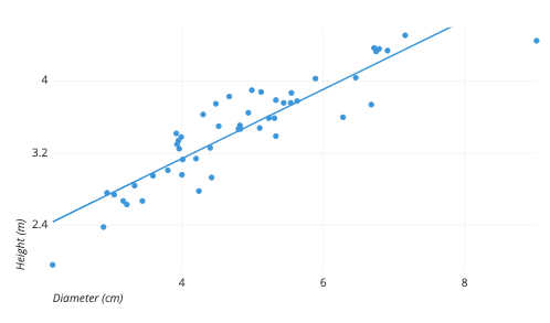
Scatter plot

Two quantitative variables

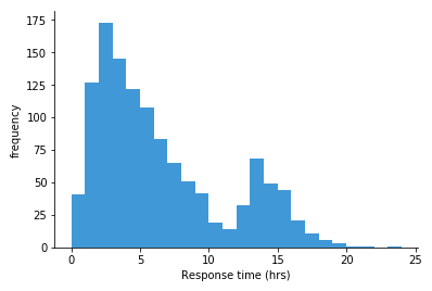
Histogram

One quantitative variable

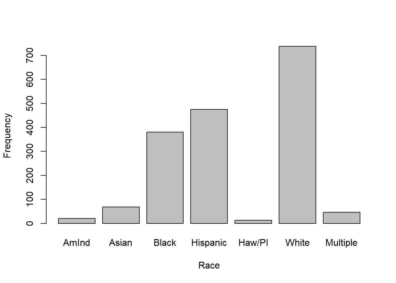
Bar plot

One categorical variable

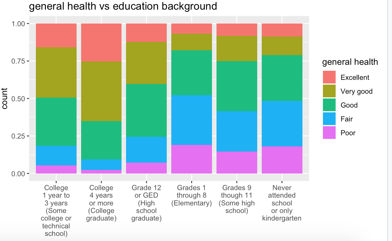
Segmented bar plot

Two categorical variables

Boxplot

One quantitative; One categorical