  > Bring a handwritten note sheet
  > Review plots
  > What does code output
  > Short answer questions
– Exam-1 (take-home)
  > released Thursday at noon
  > Open everything (except for AI)
  > Use code we have covered in class; if you have a question regarding this, please email me.
  > Due Monday at 11:59am
  > Just like the homework, a rendering issue is not an excuse to not turn in the assessment. Please render after every question.
Take-home exam
– I won’t answer any content specific questions
– I’m happy to answer any clarifying questions. Any clarifying questions asked and answered, I will make sure to re-post on Moodle for everyone
– I encourage questions! The worst thing I can do is say “I can’t help you with that”
But…
My guess is that we won’t have class on Thursday due to a chance of snow. If this is the case…
– Take home exam will still be assigned Thursday at noon
– In-class exam will be the following Tuesday (Feb-25)
Questions?
Warm-up
How can we define/understand these data types?
– <dbl>
– <int>
– <chr>
– <fct>
Warm-up
How can we define/understand these data types?
– <dbl>: means double precision, a quantitative variable that is essentially continuous - taking decimal values
– <int>: means integer, a quantitative variable that is a whole number
– <chr>: means character, contains one or a collection of characters in between quotes. Also called a string. Treated as a categorical variable in many cases
– <fct>: means factor, a categorical variable that has fixed possible values “underneath the hood”
Difference between chr and fct
Factors have additional information about the possible levels and their order, which characters do not. This is critically when you are modeling data!
Factors represent a very efficient way to store character values, because each unique character value is stored only once. This saves you a lot of computing memory when working with large data sets!
fct
The underlying value of factors corresponds to their level
fct
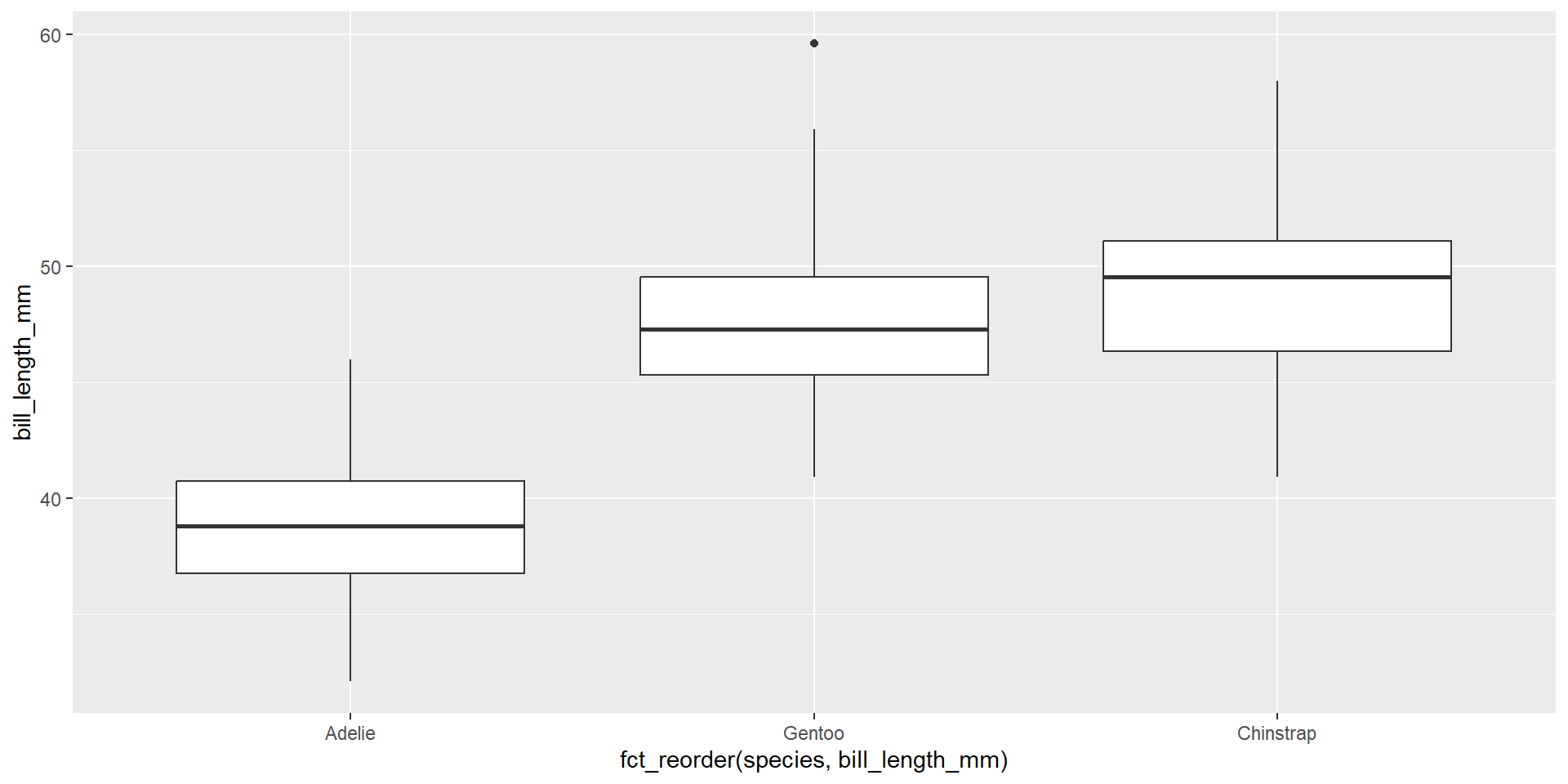
We can also take advantage of factors when plotting, through re-ordering using fct_reorder()
By default, fct_reorder uses the median. We can change this using .fun =. Change the ordering to be by max above.
So why does this work?{.smaller}
penguins |>mutate(species =as.character(species)) |>ggplot(aes(x =fct_reorder(species, bill_length_mm), y = bill_length_mm)) +geom_boxplot()
Coercion
R performs implicit coercion. This means that R automatically converts the character vector to a factor behind the scenes of the fct_reorder() function!
It’s important for us to know what R is doing, instead of treating it like a “black box”
More with data types
What is going on? How can we fix it?
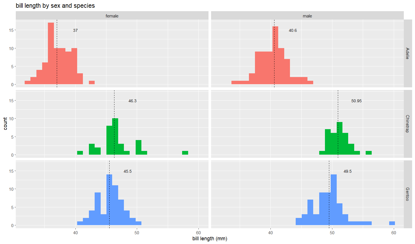
Plots
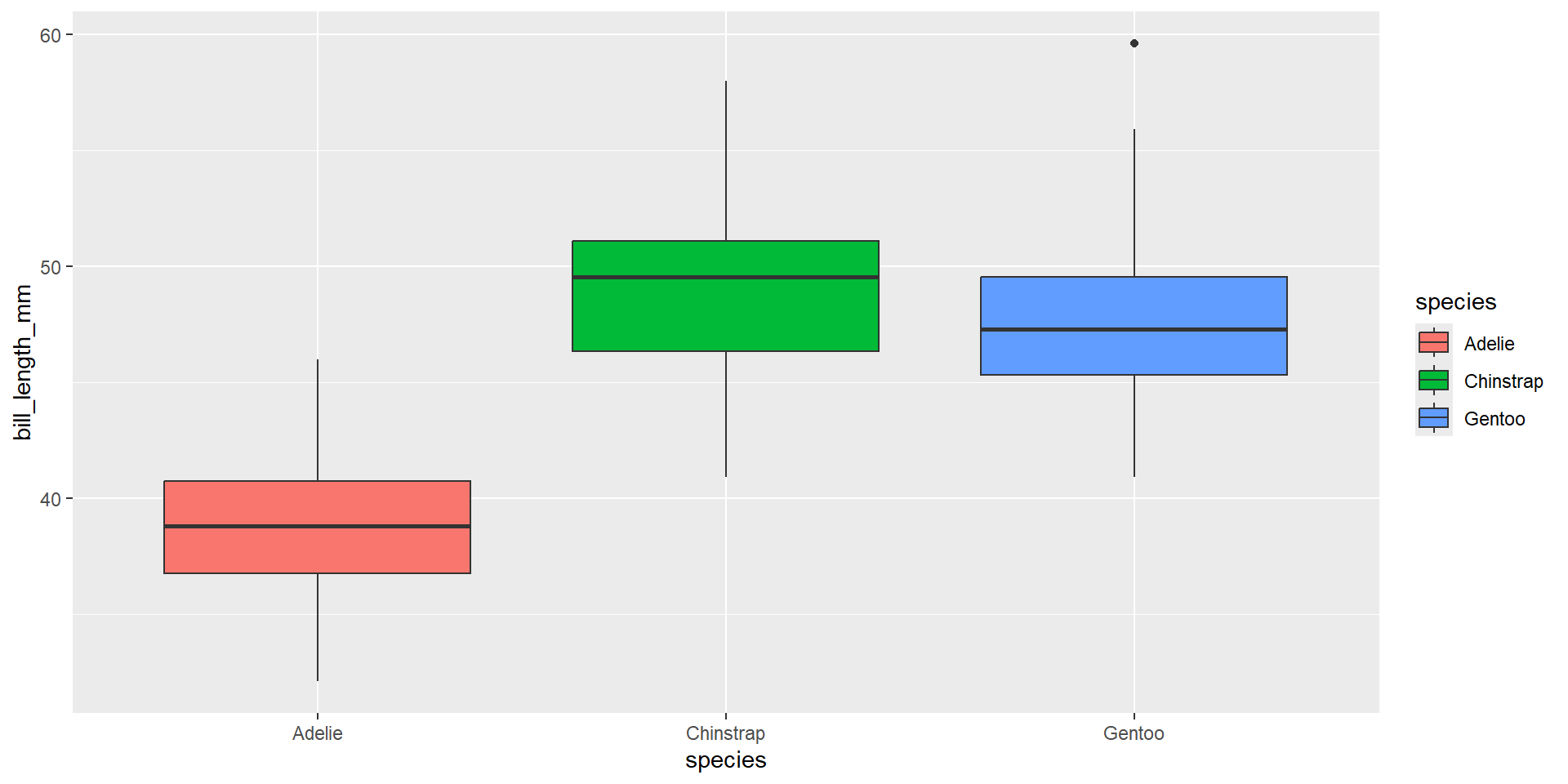
How could we improve this plot?
How could we improve this plot?
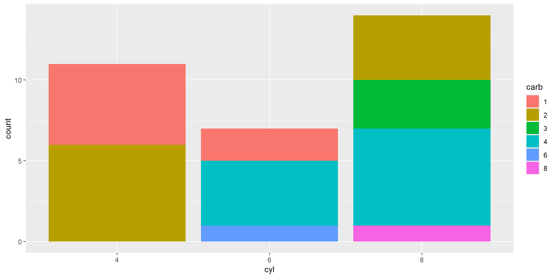
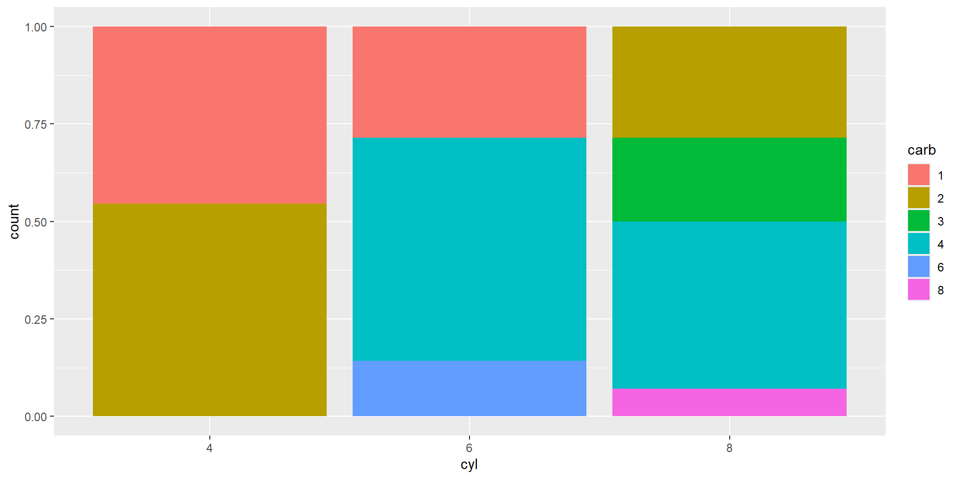
Often, we create segmented barplots to compare both within and across groups. I want us to focus specifically on the carb 4 group across the three cyl groups. What is one take away from this plot?
Note: carb = Number of carburetors; cyl = number of cylinders
In special cases, you may want to use different data sets layers onto the same plot. You can override the data + variables in a specific geom by specifying a data set and adding an aes function within a specific geom!
– If we need to create a different data set to add to our plot?
– Are there missing values?
– Explore how new geoms work
– Practice with material that is familiar
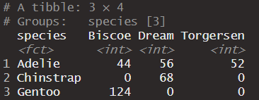
Data table
To create this, we are going to introduce replace_na()!
penguins |>filter(is.na(bill_length_mm))
# A tibble: 2 × 8
  species island    bill_length_mm bill_depth_mm flipper_length_mm body_mass_g
  <fct>   <fct>              <dbl>         <dbl>             <int>       <int>
1 Adelie  Torgersen             NA            NA                NA          NA
2 Gentoo  Biscoe                NA            NA                NA          NA
# ℹ 2 more variables: sex <fct>, year <int>
penguins |>mutate(bill_length_mm =case_when(is.na(bill_length_mm) & species =="Adelie"~14, is.na(bill_length_mm) & species =="Gentoo"~15,TRUE~ bill_length_mm)) |>arrange(bill_length_mm)
# A tibble: 344 × 8
   species island    bill_length_mm bill_depth_mm flipper_length_mm body_mass_g
   <fct>   <fct>              <dbl>         <dbl>             <int>       <int>
 1 Adelie  Torgersen           14            NA                  NA          NA
 2 Gentoo  Biscoe              15            NA                  NA          NA
 3 Adelie  Dream               32.1          15.5               188        3050
 4 Adelie  Dream               33.1          16.1               178        2900
 5 Adelie  Torgersen           33.5          19                 190        3600
 6 Adelie  Dream               34            17.1               185        3400
 7 Adelie  Torgersen           34.1          18.1               193        3475
 8 Adelie  Torgersen           34.4          18.4               184        3325
 9 Adelie  Biscoe              34.5          18.1               187        2900
10 Adelie  Torgersen           34.6          21.1               198        4400
# ℹ 334 more rows
# ℹ 2 more variables: sex <fct>, year <int>