– Part-1 of your project due March 28th at 11:59pm
  > I will grade this within GitHub. Turning in the project means having your final version pushed. To communicate best with me, have your last committ message say "final push" or something along those lines

  > Your feedback will be found in issues. The expectation is to respond and close these issues before you turn in the next itteration
– No Homework this week (please take this time to work on your project)
– Quiz Thursday (due Monday)
Warm up
What is a slope?
What is an intercept?
What is a residual?
What is a response variable?
What is a explanatory variable?
Warm up: Notation Check
\(\hat{\beta_1}\)
\(\hat{\beta_o}\)
\(r\)
\(e_i\)
Warm up: Notation Check
\(\hat{\beta_1}\) - estimated slope
\(\hat{\beta_o}\) - estimated intercept
\(r\) - estimated correlation coefficient
\(e_i\) - residual
Last time
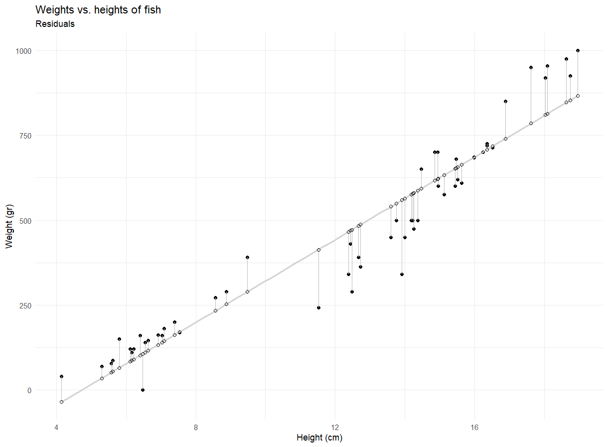
We were interested in height vs weight of fish! We fit the model using the following code:
fish_hw_fit <-linear_reg() |>fit(weight ~ height, data = fish)
Last time
Let’s use the model output to write out the estimated model using the model output
term
estimate
std.error
statistic
p.value
(Intercept)
-288.415
33.953
-8.494
0
height
60.916
2.636
23.111
0
AE
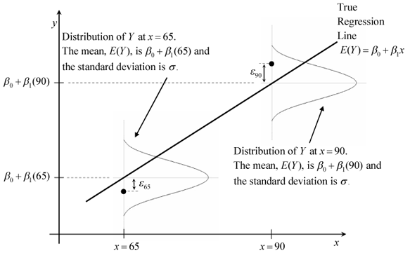
Mean response
Moving forward
> 1 Explanatory Variable
Why?
– It allows for a better understanding of the relationship between your variables
– Helps control for confounding variable
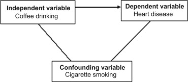
What’s a confounding variable?
Confounding variable
A confounding variable is one that has a relationship with both x and y. Including it in our model is a way to “account for it”, to get a better understanding
Simple vs Multiple Linear Regression
fish_hw_fit <-linear_reg() |>fit(weight ~ height, data = fish)tidy(fish_hw_fit) |>kable(digits =3)
term
estimate
std.error
statistic
p.value
(Intercept)
-288.415
33.953
-8.494
0
height
60.916
2.636
23.111
0
Simple vs Multiple Linear Regression
Note: There are Bream and Roach species of fish in the data set.