You have already (or will receive by today) feedback on your project… here are the next steps
Draft components
– Choose a data set
– Respond to all issues and/or close them for that data set
– Update your about section
Draft components
In your report.qmd, you are going to start writing up your report!
– Introduction and data
– Exploratory data analysis (summary stats + graphs)
– Methodology (at least the proposed idea)
  > We will have covered Simple and Multiple Linear regression by the due date
  > We will cover how to choose your "best" model + logistic regression
  > Prepare material will be posted for the remainder of the semester today
fish <-read_csv("data/fish.csv")fish_hw_fit <-linear_reg() |>fit(weight ~ height, data = fish)fish_hw_tidy <-tidy(fish_hw_fit)fish_hw_tidy |>kbl(digits =3)
term
estimate
std.error
statistic
p.value
(Intercept)
-288.415
33.953
-8.494
0
height
60.916
2.636
23.111
0
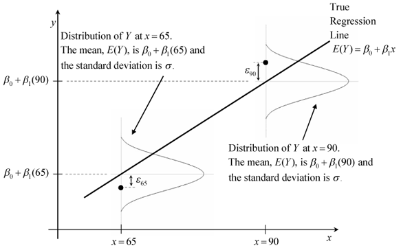
For a 1 cm increase in height, we estimate on average a 60.916 gram increase in weight
Mean response
The equation
\[
\widehat{weight} = -288.415 + 60.916*height
\]
Moving forward
> 1 Explanatory Variable
Why?
– It allows for a better understanding of the relationship between your variables
– Helps control for confounding variable
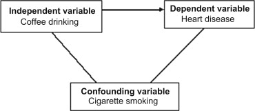
What’s a confounding variable?
Confounding variable
A confounding variable is one that has a relationship with both x and y. Including it in our model is a way to “account for it”, to get a better understanding
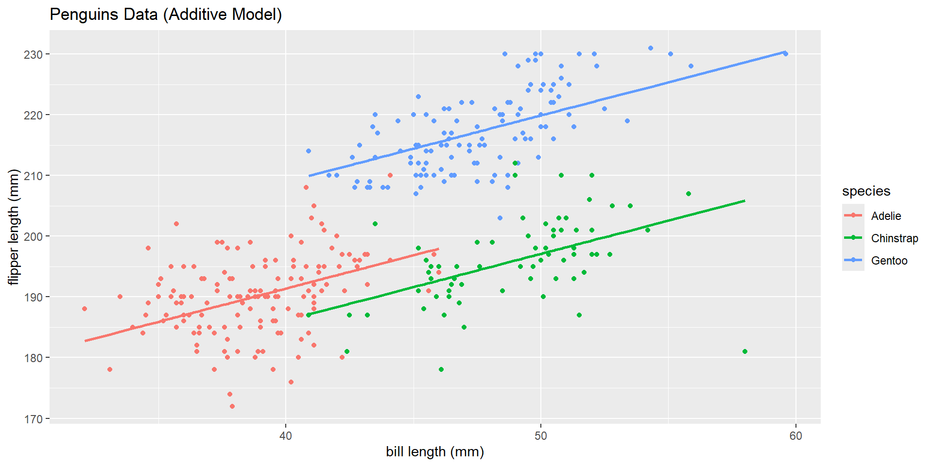
Simple vs Multiple Linear Regression
fish_hw_fit <-linear_reg() |>fit(weight ~ height, data = fish)tidy(fish_hw_fit) |>kable(digits =3)
term
estimate
std.error
statistic
p.value
(Intercept)
-288.415
33.953
-8.494
0
height
60.916
2.636
23.111
0
Simple vs Multiple Linear Regression
Note: There are Bream and Roach species of fish in the data set.