Model Selection + Assumptions + Intro to Logistic Regression

Lecture 23

Dr. Elijah Meyer

NC State University
ST 295 - Spring 2025

2025-04-10

Checklist

– We are all done with HW!

– Project draft (Apil 10th 11:59pm)

– No quiz this week

Peer Review

The Peer review instructions can be found on our website. Let’s take a look!

Warm-up

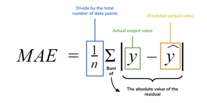
Last class, we introduced how to evaluate models using a metric called Mean Absolute Error. Walk me through this process. Specifically…

1. When would we use a metric like MAE to evaluate models?

2. How do we go about this process?

   Using the terms testing, and training data

Warm-up

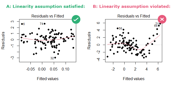
Suppose that Model 1 had a MAE of 5, and Model 2 had a MAE of 7

– What model would you say had a better predictive performance?

– Can you assume which model had more variables?

AE

Assumptions

All models have underlying assumptions that you should check for in order to trust their output. Linear regression has a few:

– Independence assumption

– Linearity assumption

– Normality assumption (more for inferential statistics)

– Constant variance (more for inferential statistics)

Independence

What does it mean to be independent?

Linearity

But what if we can’t plot it? Things get messy quick

Residual vs Fitting plot

the residuals (the difference between observed and predicted values) are plotted on the y-axis and the fitted (predicted) values are on the x-axis.

AE

Goal

Gain some exposure to logistic regression

We can’t learn everything in a week, but we can start to build a foundation

Goal

– The What, Why, and How of Logistic Regression

– How to fit these types of models in R

– How to calculate probabilities using these models

What is Logistic Regreesion

• Similar to linear regression…. but

• Modeling tool when our response is categorical

AE for motivation

Logistic regression

– This type of model is called a generalized linear model

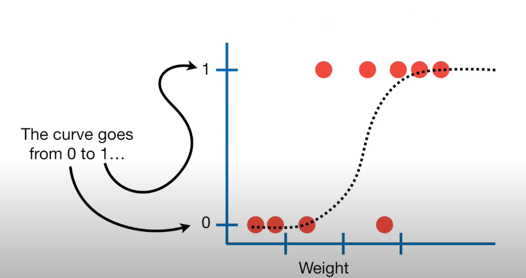
We want to fit an S curve (and not a straight line)…

where we model the probability of success as a function of explanatory a variable(s)

Problem

But linear regression fits a straight line… so we need to do something to fit that S curve…

Terms

– Bernoulli Distribution

• 2 outcomes: Success (p) or Failure (1-p)

• \(y_i\) ~ Bern(p)

• What we can do is we can use our explanatory variable(s) to model p

• Note: We use \(p_i\) for estimated probabilities

Probability

What values can probability take on?

Probability

Probabilities can take on the values of [0,1]…

Need: this means that we need to work with a model that constrains estimated probabilities (our response) to be on the correct scale [0,1]

So

p = \(\widehat{\beta_o} +\widehat{\beta}_1X1 + ....\) (bad)

so

we apply a “non-linear” transformation to the left side to fix the issue!

The transformation

The transformation is called a logit link transformation

logit(p) = \(\ln(\frac{p}{1-p})\)

\(\widehat{\ln(\frac{p}{1-p})}\) = \(\widehat{\beta_o} +\widehat{\beta}_1X1 + ....\) (good)

Breaking down the model

\(ln(\frac{p}{1-p})\) is called the logit link function, and can take on the values from \(-\infty\) to \(\infty\)

\(ln(\frac{p}{1-p})\) represents the log odds of a success

p stands for probability

This logit link function restricts p to be between the values of [0,1]

Which is exactly what we want!

Math

\(\widehat{ln(\frac{p}{1-p}})\) = \(\widehat{\beta_o} +\widehat{\beta}_1X1 + ....\)

– How do we take the inverse of a natural log?

– Taking the inverse of the logit function will map arbitrary real values back to the range [0, 1]

So

\[\widehat{ln(\frac{p}{1-p}}) = \widehat{\beta_o} +\widehat{\beta}_1X1 + ....\]

– Lets take the inverse of the logit function

– Demo Together

Final Model

\[\hat{p} = \frac{e^{\widehat{\beta_o} + \widehat{\beta_1}X1 + ...}}{1 + e^{\widehat{\beta_o} + \widehat{\beta_1}X1 + ...}}\]

Example Figure:

Recap

With a categorical response variable, we use the logit link (logistic function) to calculate the log odds of a success

\(\widehat{ln(\frac{p}{1-p})}\) = \(\widehat{\beta_o} +\widehat{\beta}_1X1 + ....\)

We can use the same model to estimate the probability of a success

\[\hat{p} = \frac{e^{\widehat{\beta_o} + \widehat{\beta_1}X1 + ...}}{1 + e^{\widehat{\beta_o} + \widehat{\beta_1}X1 + ...}}\]