Checklist
– No more HWs
– No more Quizzes
– Peer Review due tonight (11:59pm)
> My feedback will get to you by Aug 17th
– Final write up (report) & presentation due April 25th (11:59pm)
  > Moved deadline back a couple days

  > Kept review day + changed presentation format
– Final Exam (8:30am) on April 24th
  > Can bring a note sheet

  > Cumulative with very heavy emphasis on Unit 2
Logistic regression
– This type of model is called a generalized linear model
![]()
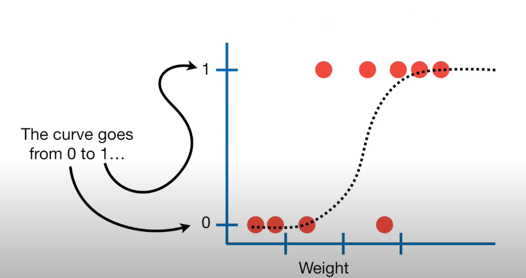
We want to fit an S curve (and not a straight line)…
where we model the probability of success as a function of explanatory a variable(s)
Problem
But linear regression fits a straight line… so we need to do something to fit that S curve…
Terms
– Bernoulli Distribution
2 outcomes: Success (p) or Failure (1-p)
\(y_i\) ~ Bern(p)
What we can do is we can use our explanatory variable(s) to model p
Note: We use \(p_i\) for estimated probabilities
Probability
What values can probability take on?
Probability
Probabilities can take on the values of [0,1]…
Need: this means that we need to work with a model that constrains estimated probabilities (our response) to be on the correct scale [0,1]
So
p = \(\widehat{\beta_o} +\widehat{\beta}_1X1 + ....\) (bad)
so
we apply a “non-linear” transformation to the left side to fix the issue!
Breaking down the model
\(ln(\frac{p}{1-p})\) is called the logit link function, and can take on the values from \(-\infty\) to \(\infty\)
\(ln(\frac{p}{1-p})\) represents the log odds of a success
p stands for probability
This logit link function restricts p to be between the values of [0,1]
Which is exactly what we want!
Math
\(\widehat{ln(\frac{p}{1-p}})\) = \(\widehat{\beta_o} +\widehat{\beta}_1X1 + ....\)
– How do we take the inverse of a natural log?
– Taking the inverse of the logit function will map arbitrary real values back to the range [0, 1]
So
\[\widehat{ln(\frac{p}{1-p}}) = \widehat{\beta_o} +\widehat{\beta}_1X1 + ....\]
– Lets take the inverse of the logit function
– Demo Together
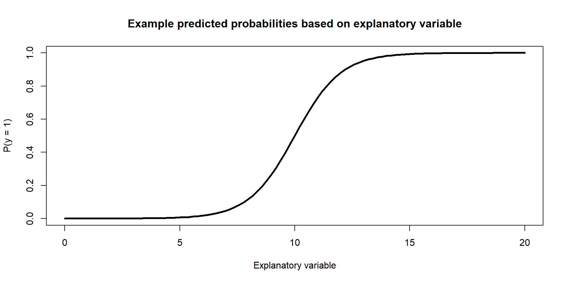
Final Model
\[\hat{p} = \frac{e^{\widehat{\beta_o} + \widehat{\beta_1}X1 + ...}}{1 + e^{\widehat{\beta_o} + \widehat{\beta_1}X1 + ...}}\]
Example Figure:
![]()
Test + Training Data Sets (Review)
A full data set is broken up into two parts
– Training Data Set
– Testing Data Set
Test + Training Data Sets
– Training Data Set - the initial dataset that you fit your model on
– Testing Data Set - the dataset that you test your model on
In R
split <- initial_split(data.set, prop = 0.80)

train_data <- training(split)
test_data <- testing(split)
If our model is doing well… we would want it to …
– predict a success when we actually observe a success
– predict a failure when we actually observe a failure
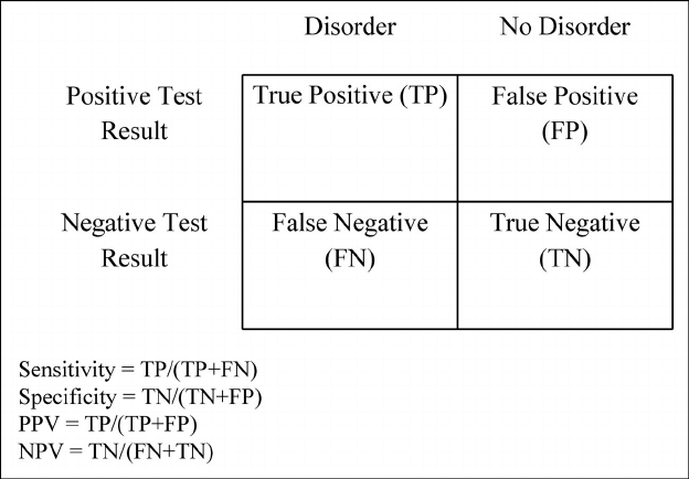
Sensitivity and Specificity
– Given that the email was actually spam, what is the probability that our model predicted the email to be spam? (Sensitivity)
– Given that the email was not spam, what is the probability that our model predicted the email to not be spam? (Specificity)
The steps
– Fit a model on the training data set (just like linear regression)
– Calculate predictions using x from the testing data set (just like linear regression)
– Compare y from the testind data set vs the predictions (just like linear regression)
> But now instead of MAE, we are going to look at specificity and sensitivity