| island | mean_fl |
|---|---|
| Biscoe | 209.71 |
| Dream | 193.07 |
| Torgersen | 191.20 |
Logistic Regression
Lecture 26
Dr. Elijah Meyer
NC State University
ST 295 - Spring 2025
2025-04-17
Checklist
– No more HWs
– No more Quizzes
– Peer Review
> My feedback will get to you by Aug 17th
– Final write up (report) & presentation due April 25th (11:59pm)
  > Moved deadline back a couple days

  > Kept review day + changed presentation format
– Final Exam (8:30am) on April 24th
  > Can bring a note sheet

  > "Cumulative" with very very heavy emphasis on Unit 2
– Statistics experience due April 22nd (11:59pm)
Tuesday Review
I want to make content around what you want to study! Please email me by Friday (5:00pm) with topic(s) you would like to see for Tuesday!
  > SLR
  > MLR
  > Logistic
Interpret model output?
Interpret graphs?
Evaluating models?
Course evaluations
Can be found here
Review
Suppose I was interested in predicting what island a penguin was on based on their flipper length. Could I use logistic regression to help answer this question?
Logistic Regression Review
Let’s assume we only want to look at Biscoe and Dream island penguins. We fit a logistic regression model and the estimates can be seen below. Let’s write out the estimated model. How can we interpret these coefficients?
      (Intercept) flipper_length_mm
       21.5153784        -0.1086004
log-odds
The log odds is the ln of the odds!
\[ odds = \frac{p}{1-p} \]
\[ logit(p) = ln(\frac{p}{1-p}) \]
– the log odds are negative if the odds are less than 1 (probability < 0.5)
– the log odds are 0 if the odds are equal to 1 (probability = 0.5)
– the log odds are positive if the odds are greater than 1 (probability > 0.5)
Probability
log odds are (generally) hard to make practical conclusions from, so we tend to answer logistic regression questions in terms of probability
\[\hat{p} = \frac{e^{\widehat{\beta_o} + \widehat{\beta_1}X1 + ...}}{1 + e^{\widehat{\beta_o} + \widehat{\beta_1}X1 + ...}}\]
Note: There isn’t an agreed upon notation for estimated probability
Evaluating these models
Test + Training Data Sets (Review)
A full data set is broken up into two parts
– Training Data Set
– Testing Data Set
Test + Training Data Sets
– Training Data Set - the initial dataset that you fit your model on
– Testing Data Set - the dataset that you test your model on
In R
split <- initial_split(data.set, prop = 0.80)

train_data <- training(split)
test_data <- testing(split)
If our model is doing well… we would want it to …
– predict a success when we actually observe a success
– predict a failure when we actually observe a failure
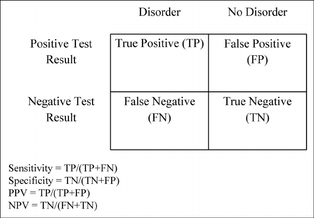
Sensitivity and Specificity
– Given that the email was actually spam, what is the probability that our model predicted the email to be spam? (Sensitivity)
– Given that the email was not spam, what is the probability that our model predicted the email to not be spam? (Specificity)
Quick probability review (doc)
The steps
– Fit a model on the training data set (just like linear regression)
– Calculate predictions using x from the testing data set (just like linear regression)
– Compare y from the testind data set vs the predictions (just like linear regression)
> But now instead of MAE, we are going to look at specificity and sensitivity
AE
Recap
With a categorical response variable, we use the logit link (logistic function) to calculate the log odds of a success
\(\widehat{ln(\frac{p}{1-p})}\) = \(\widehat{\beta_o} +\widehat{\beta}_1X1 + ....\)
We can use the same model to estimate the probability of a success
\[\hat{p} = \frac{e^{\widehat{\beta_o} + \widehat{\beta_1}X1 + ...}}{1 + e^{\widehat{\beta_o} + \widehat{\beta_1}X1 + ...}}\]