Summary Statistics + Plots

Author

Packages

library(tidyverse)

Warning: package 'ggplot2' was built under R version 4.3.3

Warning: package 'tidyr' was built under R version 4.3.3

Warning: package 'readr' was built under R version 4.3.3

Warning: package 'dplyr' was built under R version 4.3.3

Warning: package 'stringr' was built under R version 4.3.3

Warning: package 'lubridate' was built under R version 4.3.3

library(palmerpenguins)

Summary Statistics

Pull up the help file for summarise using ?summarise in the Console. Read about the description, useful functions, and then scroll down to the examples. Copy the first example in the code chunk below and run it. What is is doing? Practice reading this code as a sentence!

Note There are two different pipes in R: |> and %>%. They have identical functionality for the scope of this course. I will be using the |> pipe, as it has some computational benefits beyond the scope of 295.

mtcars |>
  summarise(mean_disp = mean(disp), n = n())

  mean_disp  n
1  230.7219 32

note: we should not name column names the same names as common functions

Now, let’s go through the second example together! Let’s comment out the code.

mtcars |> # data set and
  group_by(cyl) |> #group the data by cyl
  summarise(mean_displacement = mean(disp), n_count = n()) #calculate summary stats

# A tibble: 3 × 3
    cyl mean_displacement n_count
  <dbl>             <dbl>   <int>
1     4              105.      11
2     6              183.       7
3     8              353.      14

What happens when we group by more than one variable? Copy the code from above into the code chunk below, and also group by the vs variable. Comment on what happens.

mtcars |> # data set and
  group_by(cyl, vs) |> #group the data by cyl and vs
  summarise(mean_displacement = mean(disp), n_count = n()) #calculate summary stats```

`summarise()` has grouped output by 'cyl'. You can override using the `.groups`
argument.

# A tibble: 5 × 4
# Groups:   cyl [3]
    cyl    vs mean_displacement n_count
  <dbl> <dbl>             <dbl>   <int>
1     4     0              120.       1
2     4     1              104.      10
3     6     0              155        3
4     6     1              205.       4
5     8     0              353.      14

On your own

Create a code chunk, and use some of the useful functions in the summarise help file to calculate summary statistics using the mtcars data set.

Shortcut for code chunk Windows: ctrl + alt + I

Shortcut for code chunk Mac: cmd + option + I

mtcars |>
  summarise(mad_disp = mad(disp))

  mad_disp
1 140.4764

Data

We are going to use the penguins data set in the palmerpenguins Pull up the help file, and read more about the penguins we are going to study!

Plots

Here is a quick reference of all the different kinds of plots we can make using ggplot()! Check it out here!

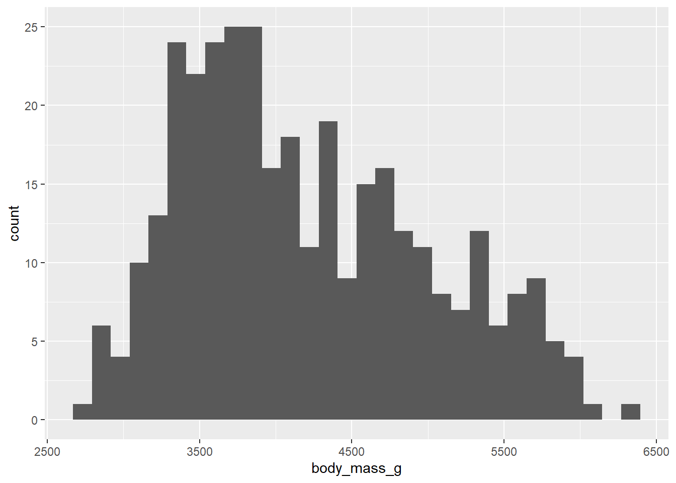
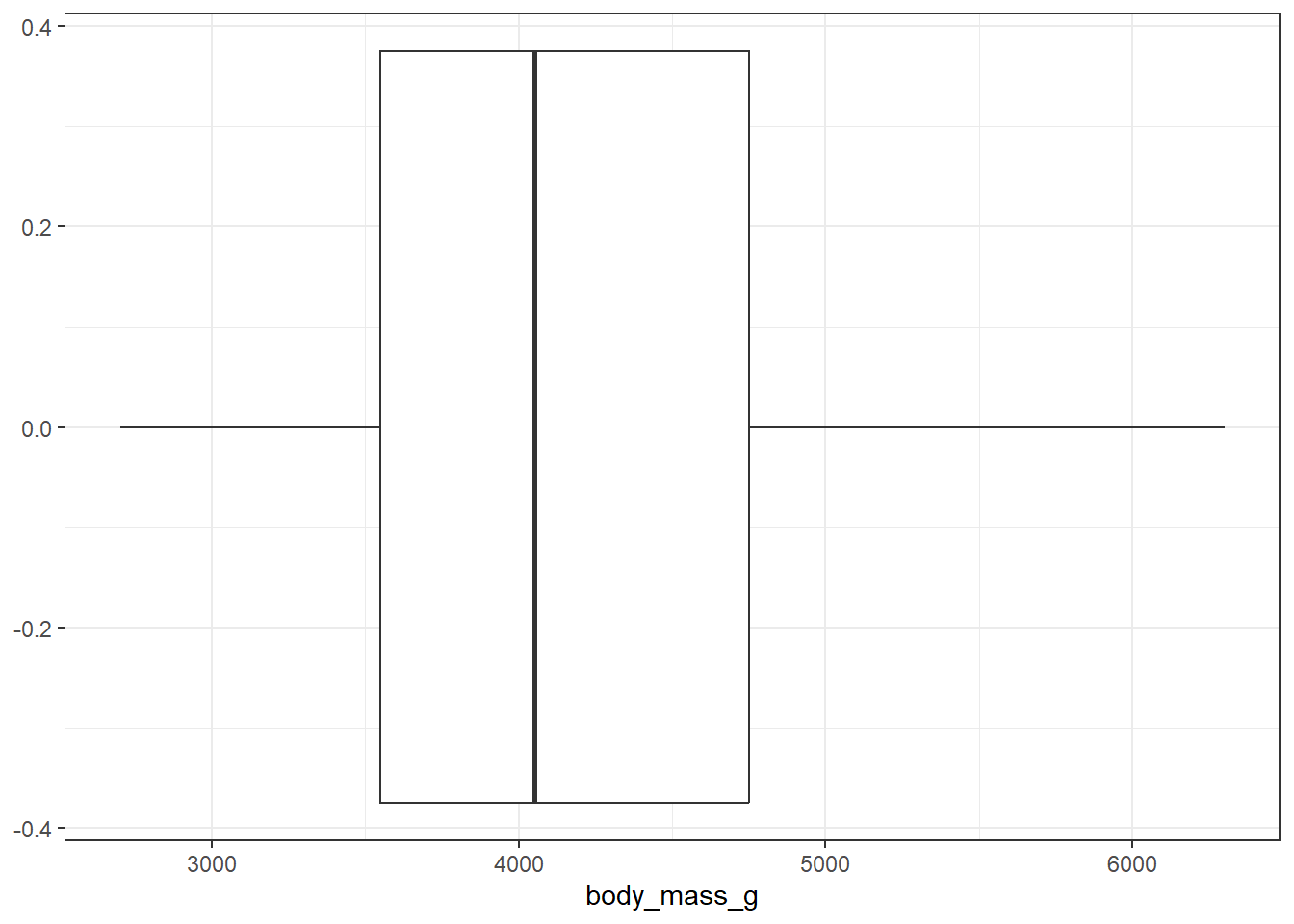
Create visualizations of the distribution of weights of penguins.

Histogram

Make a histogram by filling in the … with the appropriate arguments. Set an appropriate binwidth. Hint: you can run names(data.set) in your console if you need a quick reminder on the variable names.

To do this, we are going to use geom_histogram()

penguins |>
  ggplot( 
       aes(x = body_mass_g)) + #type variable name here
        geom_histogram()

`stat_bin()` using `bins = 30`. Pick better value with `binwidth`.

Warning: Removed 2 rows containing non-finite outside the scale range
(`stat_bin()`).

Let’s pull up the help file for that geom and talk through one of the arguments that is commonly used!

Boxplot

Now, make a boxplot of weights of penguins. To do this, we are going to use geom_boxplot()

penguins |>
  ggplot( 
       aes(x = body_mass_g)) + #type variable name here
        geom_boxplot() + 
  theme_bw()

Warning: Removed 2 rows containing non-finite outside the scale range
(`stat_boxplot()`).

Add a theme to your boxplot!

https://ggplot2.tidyverse.org/reference/ggtheme.html

Why can / should we use themes?

It’s a quick way to change the non-data aesthetics. It can make your plots look more professional!