Dplyr and Joins
Solutions
Packages
As a reminder, the dataset name is flights.
rename()
rename() changes the names of individual variables using new_name = old_name
Let’s practice using this function be renaming dep_time to departure_time.
flights |>
  rename(departure_time = dep_time) |>
  select(departure_time) # but we typically don't like spaces in names!
# A tibble: 336,776 × 1
departure_time
<int>
1 517
2 533
3 542
4 544
5 554
6 554
7 555
8 557
9 557
10 558
# ℹ 336,766 more rowsflights |>
rename("Departure Time" = dep_time) |>
select("Departure Time") # but we typically don't like spaces in names!# A tibble: 336,776 × 1
`Departure Time`
<int>
1 517
2 533
3 542
4 544
5 554
6 554
7 555
8 557
9 557
10 558
# ℹ 336,766 more rowsPractice
- Create a new dataset that only contains flights that do not have a missing departure time. Include the columns
year,month,day,dep_time,dep_delay, anddep_delay_hours(the departure delay divided by 60).
new.data <- flights |>
  filter(!is.na(dep_time)) |>
  mutate(dep_delay_hours = dep_delay / 60) |>
  select(month, day, dep_time, dep_delay, dep_delay_hours)

new.data
# A tibble: 328,521 × 5
month day dep_time dep_delay dep_delay_hours
<int> <int> <int> <dbl> <dbl>
1 1 1 517 2 0.0333
2 1 1 533 4 0.0667
3 1 1 542 2 0.0333
4 1 1 544 -1 -0.0167
5 1 1 554 -6 -0.1
6 1 1 554 -4 -0.0667
7 1 1 555 -5 -0.0833
8 1 1 557 -3 -0.05
9 1 1 557 -3 -0.05
10 1 1 558 -2 -0.0333
# ℹ 328,511 more rowsPutting it all together
We want to look at the relationship between bill length and flipper length of penguins only from the Chinstrap and Gentoo species. Further, we want to look at the relationship between bill length and flipper length after they have been scaled (divided by) body mass. On the scatter plot, fit two linear trend lines. Turn off the standard error bars.
penguins |>
  filter(species %in% c("Chinstrap", "Gentoo")) |>
  mutate(bm = bill_length_mm / body_mass_g,
         fm = flipper_length_mm / body_mass_g) |>
  ggplot(
    aes(x = bm, y = fm, colour = species)
  ) +
  geom_point() +
  geom_smooth(se = F, method = "lm")
`geom_smooth()` using formula = 'y ~ x'Warning: Removed 1 row containing non-finite outside the scale range
(`stat_smooth()`).Warning: Removed 1 row containing missing values or values outside the scale range
(`geom_point()`).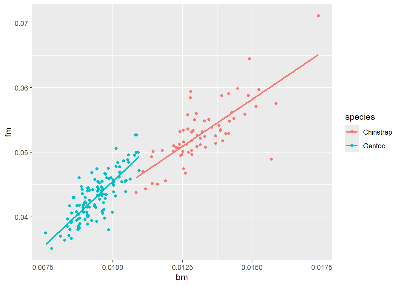
Suppose now that we want to calculate how many large Adelie penguins were observed on the Torgersen island. We consider a penguin to be large if they are larger than 4000 grams.
Hint: First, remove all the na’s from body mass.
Hint: Look up if_else()
penguins |>
  filter(species == "Adelie",
         island == "Torgersen",
         !is.na(body_mass_g)) |>
  mutate(size = if_else(body_mass_g > 4000,"large","small")) |>
  select(body_mass_g, size)
# A tibble: 51 × 2
body_mass_g size
<int> <chr>
1 3750 small
2 3800 small
3 3250 small
4 3450 small
5 3650 small
6 3625 small
7 4675 large
8 3475 small
9 4250 large
10 3300 small
# ℹ 41 more rowsBack to the slides to introduce joins!
Joins
Working with multiple data frames
Often instead of being provided the data you need for your analysis in a single data frame, you will need to bring information from multiple datasets together into a data frame yourself. These datasets will be linked to each other via a column (usually an identifier, something that links the two datasets together) that you can use to join them together.
There are many possible types of joins. All have the format something_join(x, y).
x <- tibble(
  value = c(1, 2, 3),
  xcol = c("x1", "x2", "x3")
  )

y <- tibble(
  value = c(1, 2, 4),
  ycol = c("y1", "y2", "y4")
  )

x
# A tibble: 3 × 2
value xcol
<dbl> <chr>
1 1 x1
2 2 x2
3 3 x3 y# A tibble: 3 × 2
value ycol
<dbl> <chr>
1 1 y1
2 2 y2
3 4 y4 We will demonstrate each of the joins on these small, toy datasets.
Note: These functions below know to join x and y by value because each dataset has value as a column. See for yourself!
inner_join()
inner_join(x, y)Joining with `by = join_by(value)`# A tibble: 2 × 3
value xcol ycol
<dbl> <chr> <chr>
1 1 x1 y1
2 2 x2 y2 joined data based on value numbers that appear in both
left_join()
left_join(x , y)Joining with `by = join_by(value)`# A tibble: 3 × 3
value xcol ycol
<dbl> <chr> <chr>
1 1 x1 y1
2 2 x2 y2
3 3 x3 <NA> keeps all in x and joins y
right_join()
right_join(x, y) Joining with `by = join_by(value)`# A tibble: 3 × 3
value xcol ycol
<dbl> <chr> <chr>
1 1 x1 y1
2 2 x2 y2
3 4 <NA> y4 keeps all in y and joins x
full_join()
full_join(x, y)Joining with `by = join_by(value)`# A tibble: 4 × 3
value xcol ycol
<dbl> <chr> <chr>
1 1 x1 y1
2 2 x2 y2
3 3 x3 <NA>
4 4 <NA> y4 keeps all x and y
semi_join()
semi_join(x, y)Joining with `by = join_by(value)`# A tibble: 2 × 2
value xcol
<dbl> <chr>
1 1 x1
2 2 x2 x that matches with y
anti_join()
stuff in x that is not in y