Quarto and Dates

Note: This lesson demonstrated many different code chunk options used in Quarto that can not be shown in a stagnant solutions document. Please see the video for the demonstrations!

Packages

library(tidyverse)
library(readr)
library(nycflights13)

Last Time

Last class, we worked with a flights data set. Specifically, we …

– Created a new data frame with a data type

– plotted the data with geom_freqpoly()

flights_dt <- flights |>
  select(year, month, day, hour, minute) |>
  mutate(departure = make_datetime(year, month, day, hour, minute))

flights_dt |> 
  filter(departure < as.Date("2013-01-02")) |> 
  ggplot(aes(x = departure)) + 
  geom_freqpoly(binwidth = 600)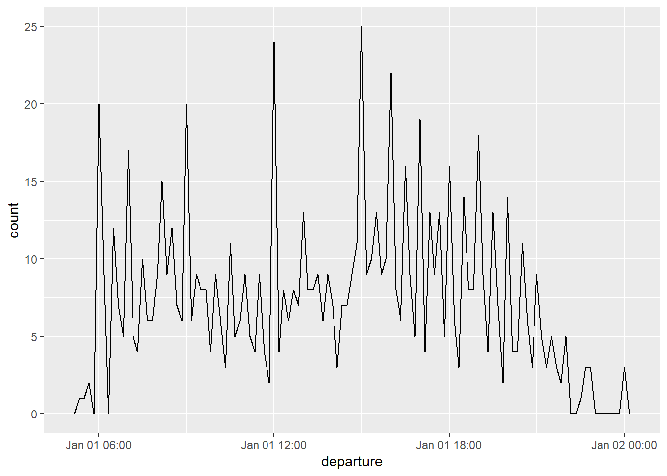

flights_dt |> 
  filter(between(departure, ymd(20130101), ymd(20130104))) |>
  ggplot(aes(x = departure)) +
  geom_freqpoly(binwidth = 600)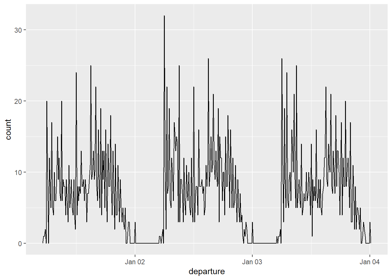

The ?@fig-plot was made using geom_freqpoly().

Try it: We could also use as.Date() on a character string instead of ymd.

Note: we tend to use <, >, or functions such as between() when working with complex data structures. Common filtering methods (ex. %in%) do not work with such a complex data structure.

Let’s make the same plot, but filter for the dates between Jan 1st and Jan 4th.

between() is a function we can nest with filter() to accomplish this!

Plot aspects in rendered document

In this section, we will introduce how to use code-chunk options to control different aspects on your plot. Specifically…

– The height of your plot #| fig-height

– The width of your plot #| fig-width

– Caption your plot #| fig-cap

– Align your plot #| fig-align

– Label your plot, and use label in your document #| label

Code chunks for the entire document

We can customize output from executed code globally, or per code block. TO this point, we have learned how to do this inside each code block. If we want to do this globally (for the entire document), we can use the execute: option in our YAML. Spacing will be important here. Under the title, let’s add

execute: echo: false

Notice the indentation. Let’s now render are code and see what happened?

We can use many code chunk options! Check out the resource here

Can we override this?

Yes! With arguments in the individual code chunk

Putting it together exercise

This part of our activity is going to challenge your problem solving skills in combination with your coding skills

Road Casualties in Great Britain 1969–84

UKDriverDeaths is a time series giving the monthly totals of car drivers in Great Britain killed or seriously injured Jan 1969 to Dec 1984. Compulsory wearing of seat belts was introduced on 31 Jan 1983. This is a pre-loaded data frame in R called UKDriverDeaths.

Below, let’s start by getting these data into a much more workable format. Let’s name the new data set full_data. We want a data set that has the number of driver deaths, month, and year. In addition, create a date variable with the data type date that has.

Hint: We are going to take advantage of rep() to make some variables. What does rep() do?

year_date <- c(1969, 1970, 1971, 1972, 1973, 1974, 1975, 1976, 1977, 1978, 1979, 1980, 1981, 1982, 1983, 1984)

UKDriverDeaths |>
  tibble() |>
  rename(driver_deaths = UKDriverDeaths) |>
  mutate(month = rep(1:12, 16),
         year = rep(year_date, each = 12),
         date = make_date(year,month))

# A tibble: 192 × 4
   driver_deaths month  year date      
           <dbl> <int> <dbl> <date>    
 1          1687     1  1969 1969-01-01
 2          1508     2  1969 1969-02-01
 3          1507     3  1969 1969-03-01
 4          1385     4  1969 1969-04-01
 5          1632     5  1969 1969-05-01
 6          1511     6  1969 1969-06-01
 7          1559     7  1969 1969-07-01
 8          1630     8  1969 1969-08-01
 9          1579     9  1969 1969-09-01
10          1653    10  1969 1969-10-01
# ℹ 182 more rows

We will make the plot when you come back from Spring Break!