Review and Words: Solutions
Packages
Putting it together exercise
This part of our activity is going to challenge your problem solving skills in combination with your coding skills
Road Casualties in Great Britain 1969–84
UKDriverDeaths is a time series giving the monthly totals of car drivers in Great Britain killed or seriously injured Jan 1969 to Dec 1984. Compulsory wearing of seat belts was introduced on 31 Jan 1983. This is a pre-loaded data frame in R called UKDriverDeaths.
UKDriverDeaths Jan Feb Mar Apr May Jun Jul Aug Sep Oct Nov Dec
1969 1687 1508 1507 1385 1632 1511 1559 1630 1579 1653 2152 2148
1970 1752 1765 1717 1558 1575 1520 1805 1800 1719 2008 2242 2478
1971 2030 1655 1693 1623 1805 1746 1795 1926 1619 1992 2233 2192
1972 2080 1768 1835 1569 1976 1853 1965 1689 1778 1976 2397 2654
1973 2097 1963 1677 1941 2003 1813 2012 1912 2084 2080 2118 2150
1974 1608 1503 1548 1382 1731 1798 1779 1887 2004 2077 2092 2051
1975 1577 1356 1652 1382 1519 1421 1442 1543 1656 1561 1905 2199
1976 1473 1655 1407 1395 1530 1309 1526 1327 1627 1748 1958 2274
1977 1648 1401 1411 1403 1394 1520 1528 1643 1515 1685 2000 2215
1978 1956 1462 1563 1459 1446 1622 1657 1638 1643 1683 2050 2262
1979 1813 1445 1762 1461 1556 1431 1427 1554 1645 1653 2016 2207
1980 1665 1361 1506 1360 1453 1522 1460 1552 1548 1827 1737 1941
1981 1474 1458 1542 1404 1522 1385 1641 1510 1681 1938 1868 1726
1982 1456 1445 1456 1365 1487 1558 1488 1684 1594 1850 1998 2079
1983 1494 1057 1218 1168 1236 1076 1174 1139 1427 1487 1483 1513
1984 1357 1165 1282 1110 1297 1185 1222 1284 1444 1575 1737 1763head(UKDriverDeaths)[1] 1687 1508 1507 1385 1632 1511Below, let’s start by getting these data into a much more workable format. Let’s name the new data set full_data. We want a data set that has the number of driver deaths, month, and year. In addition, create a date variable with the data type date that has.
Hint: We are going to take advantage of rep() to make some variables. What does rep() do?
To make this plot, we are going to introduce:
and review
If you could not create the full_data object, it is down below!
full_data |>
  filter(date < ymd(19700101)) |>
  ggplot(
    aes(x = date, y = driver_deaths)
  ) +
  geom_line(color = "black", lwd = 2) +
  geom_area(fill = "lightblue") +
  scale_x_date(date_breaks = "2 month", date_labels = "%Y/%m") +
  scale_y_continuous(limits = c(0, 3000)) +
  labs(title = "Road Casualities in Great Britain 1969",
       y = "driver deaths",
       x = "")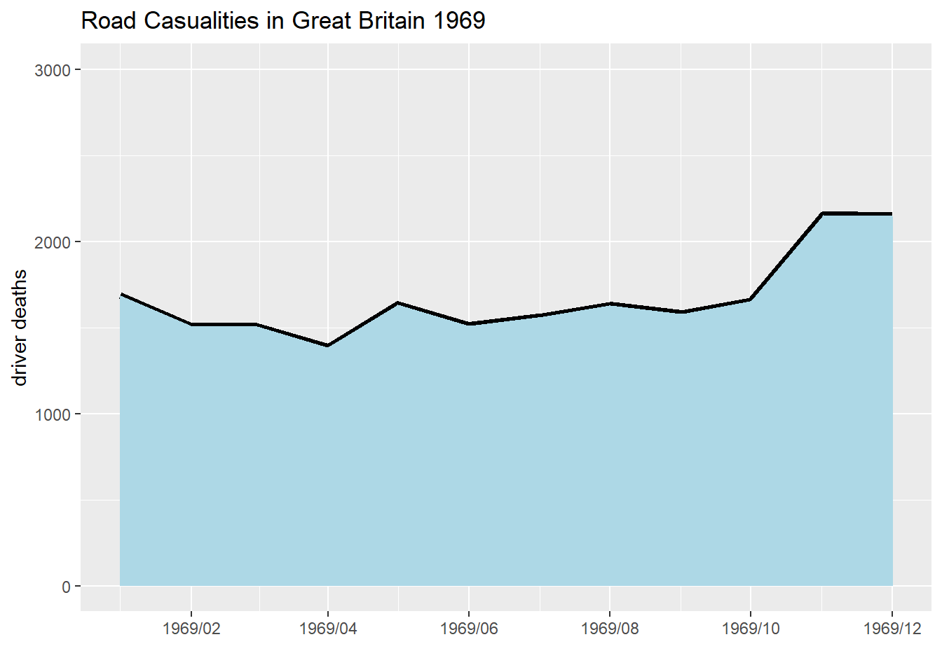
================================
Working with Qualititive Data
For this activity, we are going to work with the friends data set. This package is not pre-installed for us, and we need to install it ourselves using install.packages("friends"). Should this go in the Console or our .qmd file?
Now, install the package, and write the code to library it below:
# A tibble: 6 × 6
  text                                    speaker season episode scene utterance
  <chr>                                   <chr>    <int>   <int> <int>     <int>
1 There's nothing to tell! He's just som… Monica…      1       1     1         1
2 C'mon, you're going out with the guy! … Joey T…      1       1     1         2
3 All right Joey, be nice. So does he ha… Chandl…      1       1     1         3
4 Wait, does he eat chalk?                Phoebe…      1       1     1         4
5 (They all stare, bemused.)              Scene …      1       1     1         5
6 Just, 'cause, I don't want her to go t… Phoebe…      1       1     1         6
Once you do this, you should be able to explore the friends data set. First let’s pull up the help file. Note: an utterance is a spoken word, statement, or vocal sound.
We are going to explore which character loves (said?) coffee the most!
For this, we are going to use the function str_detect(). Specifically, we are going to subset our rows that only have the word coffee in an utterance. Let’s save this as a new R object, friends_coffee.
friends |>
  filter(str_detect(text, fixed("coffee", ignore_case = TRUE)))
# A tibble: 286 × 6
text speaker season episode scene utterance
<chr> <chr> <int> <int> <int> <int>
1 Let me get you some coffee. Monica… 1 1 1 28
2 Can I get you some coffee? Waitre… 1 1 1 50
3 Isn't this amazing? I mean, I have ne… Rachel… 1 1 11 1
4 Y'know, I figure if I can make coffee… Rachel… 1 1 11 4
5 Come on, you made coffee! You can do … Ross G… 1 1 14 13
6 Would anybody like more coffee? Rachel… 1 1 15 11
7 Yeah. Yeah, I'll have a cup of coffee. #ALL# 1 1 15 14
8 Ahh, miss? More coffee? Custom… 1 1 15 16
9 Alright, don't tell me, don't tell me… Rachel… 1 3 3 5
10 They wanna know if I'm okay. Okay.. t… Rachel… 1 4 5 12
# ℹ 276 more rows