library(tidyverse)
library(tidymodels)
library(scatterplot3d)
library(palmerpenguins)Additive models
Solutions
Load packages and data
Today
By the end of this week…
- understand the difference between and additive vs interaction model
- be able to build, fit and interpret linear models with \(>1\) predictor
- think critically about r-squared as a model selection tool
Penguins
We are going to work with the Penguins data set for this example so we can get some coding practice + conceptual practice. As a researcher, you are really interested in flipper length (y), and think bill length (x) could be a useful predictor for your model. Why might you also want to include species in the model?
because species may be a confounding variable (relationship with both flipper length and bill length)
Fitting the additive model
To fit the additive model, we can use the + sign. Do this below.
model1 <- linear_reg() |>
  fit(flipper_length_mm ~ bill_length_mm + species, data = penguins)

tidy(model1)
# A tibble: 4 × 5
term estimate std.error statistic p.value
<chr> <dbl> <dbl> <dbl> <dbl>
1 (Intercept) 148. 4.17 35.4 6.78e-116
2 bill_length_mm 1.08 0.107 10.1 3.12e- 21
3 speciesChinstrap -5.00 1.37 -3.65 3.00e- 4
4 speciesGentoo 17.8 1.17 15.2 3.45e- 40Write
Let’s use LaTeX to write out the model in proper notation. This includes defining and understanding what an indicator function is! Let’s do this together.
\[ \widehat{flipper} = 148 + 1.08*bill - 5*chinstrap + 17.8*gentoo \]
The estimates for chinstrap and gentoo are deviations from a baseline group (Adelie) <- R picked this because it comes first in the alphabet
Adelie
\[ \widehat{flipper} = 148 + 1.08*bill - 5*0 + 17.8*0 \]
\[ \widehat{flipper} = 148 + 1.08*bill \]
Gentoo \[ \widehat{flipper} = 148 + 1.08*bill - 5*0 + 17.8*1 \]
\[ \widehat{flipper} = 148 + 17.8 + 1.08*bill \]
Where is the baseline? It’s the intercept
\[ Gentoo= \begin{cases} \text{1 if penguin is Gentoo}\\ \text{0 if else} \end{cases} \]
\[ Chinstrap= \begin{cases} \text{1 if penguin is Chinstrap}\\ \text{0 if else} \end{cases} \]
Draw
Draw it out. Based on the model output, what would this model look like?
An additive model for MLR assumes that the relationship between bill length and flipper length does not change based on species
Prediction using R
Let’s use R to make predictions using this additive model. Use R to predict the flipper length for a Gentoo penguin that has a bill length of 60.
predict(model1, data.frame(bill_length_mm = 60, species = "Gentoo"))# A tibble: 1 × 1
.pred
<dbl>
1 231.Interpretation
Now, let’s interpret these coefficients in the context of the problem:
Intercept: For a bill length of 0, we estimate the mean flipper length of the Adelie penguins to be 148mm
speciesChinstrap: Holding bill length constant, we estimate the mean flipper length of the Chinstap penguins to be 5mm less than the Adelie penguins
bill_length_mm: After accounting for species (holding species constant)… for a 1 mm increase in bill length, we estimate on average an increase in flipper length by 1.08mm
Can we do this with 2 quantitative variables?
Yes! Let’s look at the explanatory variables bill length (mm) and body mass (g).
The concept is the same, the picture is a bit different! What about, instead of species, we wanted to use body_mass_g. Note, the following code is to help us understand the material, and is not a learning objective of the course. The code you need to know is lm.
s3d <- penguins |>
  dplyr::select(bill_length_mm, body_mass_g, flipper_length_mm) |>
  scatterplot3d(xlab = "bill length (mm)",
                ylab = "body mass (g)",
                zlab = "flipper length (mm)",
                main = "additive model with 2 quan variables")
Warning: Unknown or uninitialised column: `color`.model2 <- lm(flipper_length_mm ~ bill_length_mm + body_mass_g, penguins)
s3d$plane3d(model2)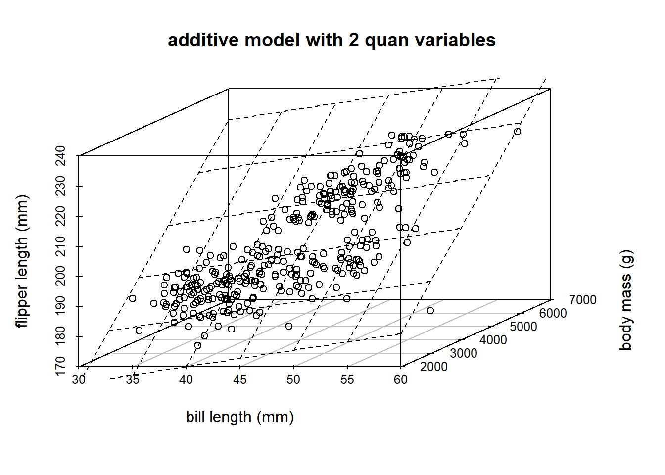
               Estimate Std. Error t value Pr(>|t|)
(Intercept)     121.956      2.855  42.715        0
bill_length_mm    0.549      0.080   6.859        0
body_mass_g       0.013      0.001  23.939        0