Interaction Model + R-squared: Solutions

Load packages and data

library(tidyverse)
library(tidymodels)
library(palmerpenguins)
library(yardstick)

Today

By the end of today you will…

• be able to build, fit and interpret linear models with \(>1\) predictor
• think critically about r-squared as a model selection tool
• use adjusted r-squared to compare models

Interaction model

We are going to continue working with the penguins data set. Last class, we fit the additive model between flipper length, bill length, and species. Now, let’s fit the interaction model. Name this model_int. Provide the summary output. Before we fit it, let’s visualize it!

Note: What does the interaction model allow us to have that the additive model doesn’t?

it allows the relationship between x and y to change based on the values of z

penguins |>
  ggplot(
    aes(x = bill_length_mm, y = flipper_length_mm, colour = species)
  ) +
  geom_point() +
  geom_smooth(method = "lm", se = F)

`geom_smooth()` using formula = 'y ~ x'

Warning: Removed 2 rows containing non-finite outside the scale range
(`stat_smooth()`).

Warning: Removed 2 rows containing missing values or values outside the scale range
(`geom_point()`).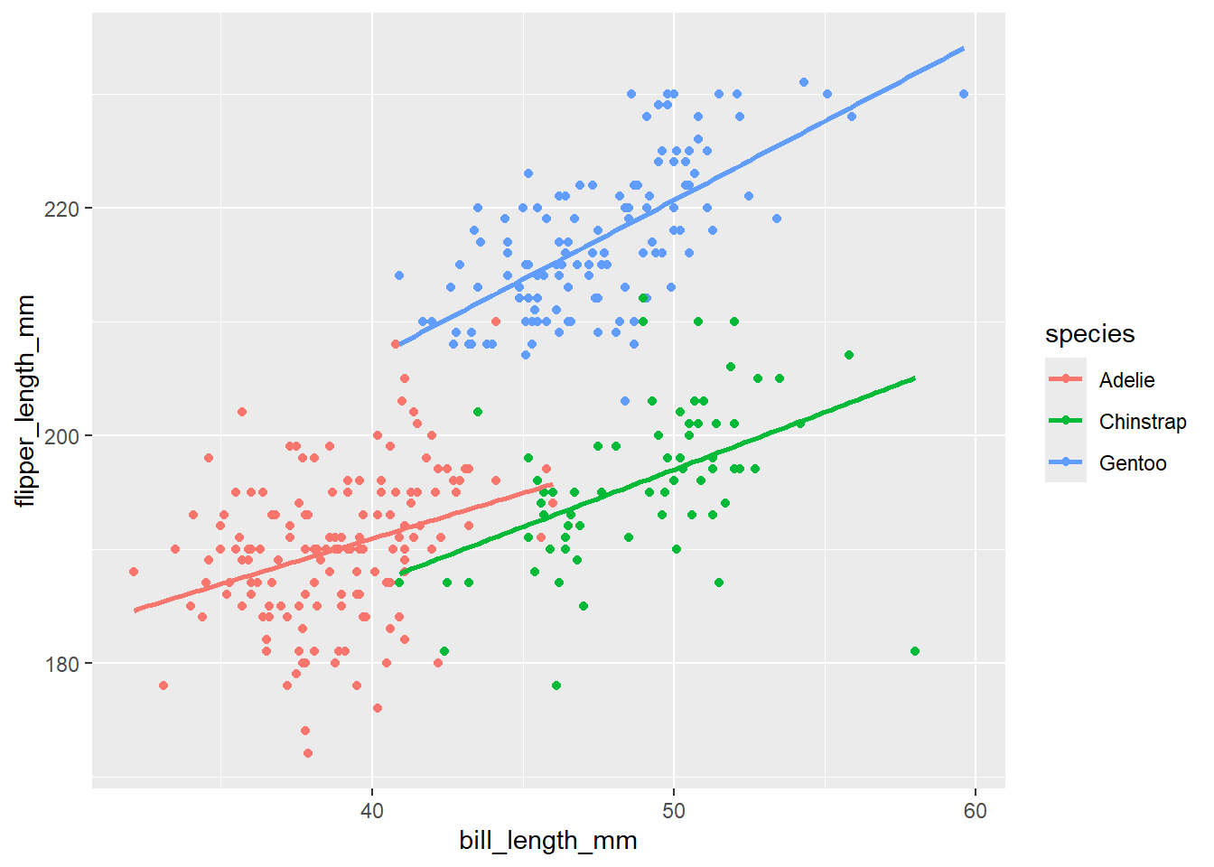

model_int <- linear_reg() |>
  fit(flipper_length_mm ~ bill_length_mm*species, data = penguins)

And just like before, we can make predictions!

predict(model_int, data.frame(bill_length_mm = 40,  species = "Adelie"))

# A tibble: 1 × 1
  .pred
  <dbl>
1  191.

Now, simplify our model for just the Chinstrap penguins, showing how both the slope and intercept change from the baseline in this interaction model.

See demo on doc-cam: take notes here

Write out the interpretation for one of the interaction coefficients here

.207 is the estimated increase in mean flipper length for Chinstrap penguins compared to Adelie penguins for a 1mm increase in bill length.

Let’s talk about r-squared

As a reminder, \(R^2\) is defined as the amount of variability in our response (y) that is explained by our model with x explanatory variable(s)

Demo

Note: There isn’t a pre-built function to calculate r-squared and adjusted r-squared using tidymodels. We could write our own, or use base R. Because you will (probably) see base R outside of this class, let’s use lm, the base R version of linear models. You can use either on HW/project.

Let’s calculate and interpret r-squared.

####### models + r.squared value

slr_model <- lm(flipper_length_mm ~ bill_length_mm, data = penguins) 

summary(slr_model)$r.squared # slr model

[1] 0.430574

add_model <- lm(flipper_length_mm ~ bill_length_mm + species, data = penguins)
summary(add_model)$r.squared # additive model

[1] 0.8298693

model_int <- lm(flipper_length_mm ~ bill_length_mm*species, data = penguins) 
summary(model_int)$r.squared # interaction model

[1] 0.8328305

Model selection

Can we use r-squared to select the best model? Let’s explore…

set.seed(12345)
random_peng <- rbeta(nrow(penguins), 20, 10) # make 100 random numbers

penguins_fake <- cbind(penguins, random_peng) # add that variable to the data

nonsense_model <- lm(flipper_length_mm ~ bill_length_mm*species*random_peng, data = penguins_fake )
summary(nonsense_model)$r.squared #interaction model with a literal random variable

[1] 0.8441509

So, can we use r-squared for model selection? Why or why not?

No! r-squared will always increase as our models get more complicated!