── Conflicts ────────────────────────────────────────── tidyverse_conflicts() ──
✖ dplyr::filter() masks stats::filter()
✖ dplyr::lag()    masks stats::lag()
ℹ Use the conflicted package (<http://conflicted.r-lib.org/>) to force all conflicts to become errors
Up through this point, we have gone through SLR and MLR. You may be asking yourself, how do we choose? There are a lot of different ways we can justify a choice of model. In this activity, we are going to justify a model based on it’s predictive performance.
The Iris data set is a pre-loaded data set in R. Pull up the help file for the Iris data set to see what it’s all about. In this case, we are interested in Sepal length, and will fit a variety of models to investigate Sepal length.
The goal of this activity is to choose a model that “performs the best” when predicting new observations.
Last time
iris_full<-iris|>mutate(id =1:nrow(iris))set.seed(123)# sample_n does not have a set.seed argument... so use this!train<-iris_full|>sample_n(.8*nrow(iris_full), replace =FALSE)test<-iris_full|>anti_join(train, by ="id")model1<-linear_reg()|># linear regfit(Sepal.Length~Sepal.Width, data =train)# y ~ xpred<-predict(model1, data.frame(Sepal.Width =test$Sepal.Width))data<-data.frame(pred, test$Sepal.Length)# y-hat, ymae(data, truth =test.Sepal.Length, estimate =.pred)
# A tibble: 1 × 3
  .metric .estimator .estimate
  <chr>   <chr>          <dbl>
1 mae     standard       0.631
Let’s compare models
Repeat the steps above, but now, fit an interaction model with the explanatory variables Petal Width and Sepal Width. Calculate the MAE. How does it compare to your SLR model?
model2<-linear_reg()|>fit(Sepal.Length~Sepal.Width*Petal.Width, data =train)pred2<-predict(model2, data.frame(Sepal.Width =test$Sepal.Width, Petal.Width =test$Petal.Width))data2<-data.frame(pred2, test$Sepal.Length)mae(data2, .pred, test.Sepal.Length)
# A tibble: 1 × 3
  .metric .estimator .estimate
  <chr>   <chr>          <dbl>
1 mae     standard       0.275
Make a decision
Model 2 does a better job at predicting sepal length than model 1
Adjusted-R-squared
What if we use adjusted-r-squared? Do we come to the same conclusions?
Maybe? Adjusted R-squared and Mean Absolute Error (MAE) are both used to evaluate regression models, but they focus on different aspects of model performance: Adjusted R-squared measures how well the model explains the variance in Y (after accounting for the number of variables in the model), while MAE measures the average magnitude of prediction errors.
Can adjusted r squared go down?
Yes, we know this to be true. Is that the case here? Compare model 2 with the SLR model and a MLR model with just an additive effect.
model1<-lm(Sepal.Length~Sepal.Width, data =iris)#SLRsummary(model1)$adj.r.square
[1] 0.007159294
model2<-lm(Sepal.Length~Sepal.Width*Petal.Width, data =iris)#intsummary(model2)$adj.r.square#.702
[1] 0.7021525
model3<-lm(Sepal.Length~Sepal.Width+Petal.Width, data =iris)#addsummary(model3)$adj.r.square#.703
[1] 0.7032539
Interaction: The relationship between sepal length (y) and sepal width (x) depends on petal width (x2)
Add: The relationship between sepal length (y) and sepal width (x) does NOT depend on petal width (x2)
Which model would you choose here?
Add model
What is Occam’s Razor (also known as the law of parsimony): The more simple model is easier to interpret
Pick the more simple model if there isn’t a big difference between the two
Are any of these models appropriate?
Let’s go to the slides!
Two things need to hold true for these models to be trustworthy:
– Independence: Checked based on how the data are collected / related to each other (independence of individual observations and NOT the variables)
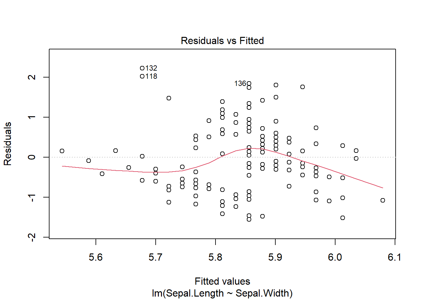
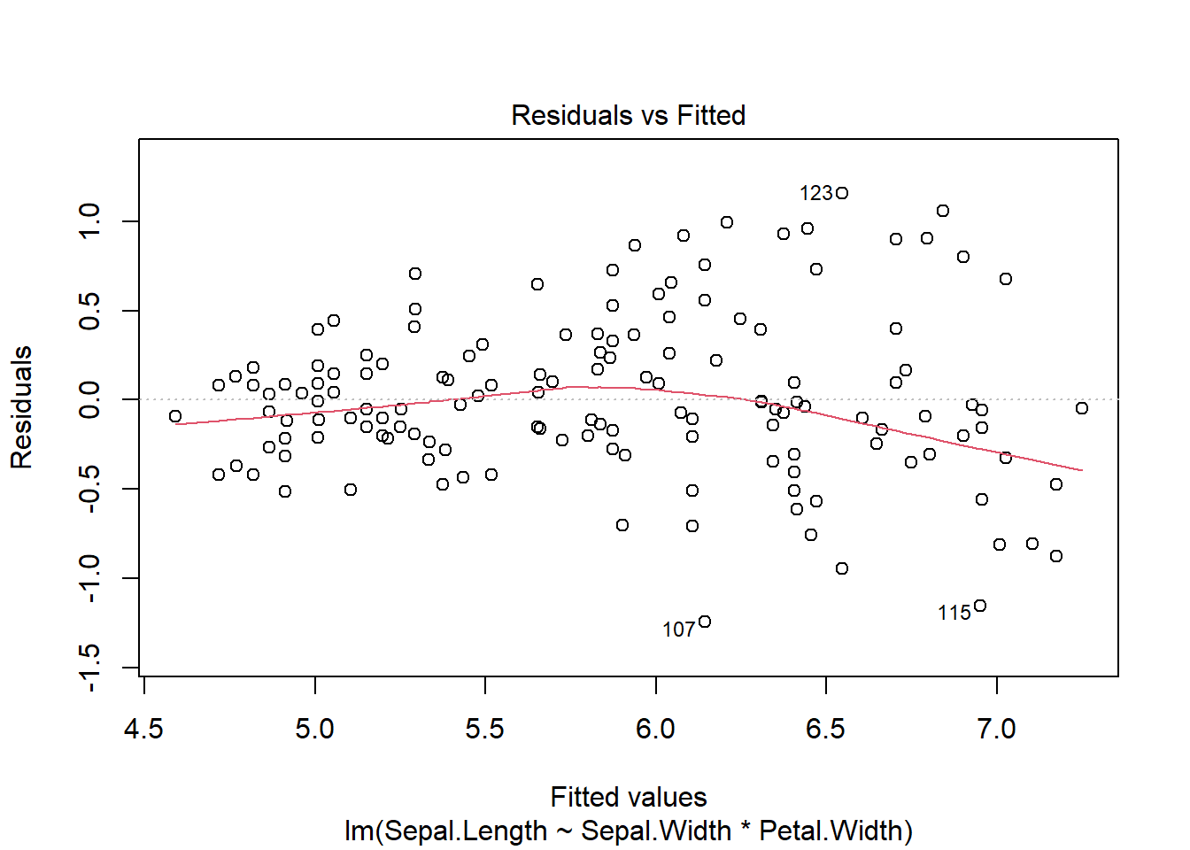
– Linearity: Take a look at residuals vs fitted and check for random scatter pattern (cloud like)
Let’s define these terms, and discuss how to check them below….
#base R with a base R lm model

plot(model1, which=c(1))