# A tibble: 56 × 3
   year  degree     n
   <chr> <chr>  <dbl>
 1 2011  AB         2
 2 2011  AB2        0
 3 2011  BS         5
 4 2011  BS2        2
 5 2012  AB         2
 6 2012  AB2        1
 7 2012  BS         9
 8 2012  BS2        6
 9 2013  AB         4
10 2013  AB2        0
# ℹ 46 more rowsMidterm - In class - Solutions
STA 295 - Spring 2025
Name: ___________________________________
I hereby state that I have not communicated with or gained information in any way from my classmates, or any external resources during this exam, and that all work is my own.
Signature: _________________________________
Any potential violation of NC State’s policy on academic integrity will be reported. All work on this exam must be your own.
- You have 75 minutes to complete the exam.
- You are allowed one \(8\frac{1}{2}" \times 11"\) sheet of notes (cheat sheet) with writing on both sides, pen or a pencil, and to ask questions to the professor.
- You are not allowed a cell phone, even if you intend to use it for checking the time, music device or headphones, notes (other than your cheat sheet), books, or other resources, or to communicate with anyone other than the professor during the exam.
- For multiple choice questions, please circle your answer.
- This is a 60 point exam. Point values per question can be found next to the question name.
Good luck!
Question 1 (4 points)
In 1-2 sentences, explain the difference between R and RStudio.
R is a statistical programming language (car engine), while RStudio is the integrated environment (IDE) (car dashboard)
Question 2 (4 points)
In 2-4 sentences, explain how GitHub can be a useful tool for statisticians, data scientists, and researchers.
GitHub is critical for reproducible work, and transparency. These are things we need to strive for as a statistics/research community. It’s also an important tool for collaboration.
Statistical Science majors
The data for this question is on Statistical Science majors at Duke over the years. The Department of Statistical Science offers two majors – Bachelor of Science (BS) and Bachelor of Arts (AB). Students who have Statistical Science as their first major are coded as BS and AB, those who have it as their second major are coded as BS2 and AB2. The data frame, statsci, is shown below. The question is on the next page.
Question 3 (3 points)
Your teammate made the following plot and took a screenshot of it, but they haven’t saved the code in your Quarto document.
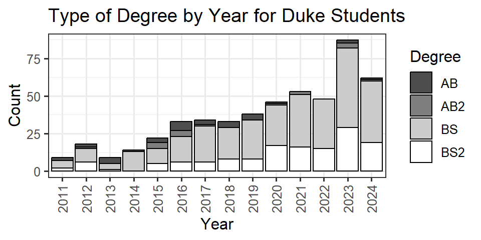
Now the whole team needs to work backwards from the plot and figure out the code that generated it. Which of the following produces the plot?
a.
ggplot(statsci, aes(x = year, y = n, fill = degree)) +
geom_col()ggplot(statsci, aes(x = degree, y = n, fill = year)) +
geom_col()ggplot(statsci, aes(x = year, y = n, fill = degree)) +
geom_bar()ggplot(statsci, aes(x = degree, y = n, fill = year)) +
geom_bar()Question 4a (3 points)
Currently, the above plot is hard to read. In 1-2 sentences, explain it would be better to display this information using relative proportions vs counts.
**The above plot is hard to read because the sample sizes across year are extremely different! It’s not the most appropriate to share data in this way when sample sizes differ across group significantly.
Question 4b (3 points)
Identify the argument, that would go inside the appropriate geom, to help fix the concern in question 4a.
position = "stack"b.
position = "fill"position = "prop"position = "size"Question 5 (2 points)
True or False: ggplot(statsci,...) is equivalent to statsci |> ggplot(...)
a. True
- False
Question 5b (2 points)
True or False: aes() is a …
a. function
- argument
Question 6 (3 points)
Another teammate has made the following table for your report. But they also haven’t saved their code for generating this table.
| degree | 2011 | 2012 | 2013 | 2014 | 2015 | 2016 | 2017 | 2018 | 2019 | 2020 | 2021 | 2022 | 2023 | 2024 |
|---|---|---|---|---|---|---|---|---|---|---|---|---|---|---|
| AB | 2 | 2 | 4 | 1 | 3 | 6 | 3 | 4 | 4 | 1 | 0 | 0 | 2 | 1 |
| AB2 | 0 | 1 | 0 | 0 | 4 | 4 | 1 | 0 | 0 | 1 | 2 | 0 | 3 | 1 |
| BS | 5 | 9 | 4 | 13 | 10 | 17 | 24 | 21 | 26 | 27 | 35 | 33 | 53 | 41 |
| BS2 | 2 | 6 | 1 | 0 | 5 | 6 | 6 | 8 | 8 | 17 | 16 | 15 | 29 | 19 |
Which of the following is the correct combination of values that should go into the blanks in the code cell below to get statsci into the right shape for this table? Note: You can revisit the original data set on page 2.
statsci |>
  pivot_wider(
    names_from = _BLANK_1_,
    values_from = _BLANK_2_
  )
BLANK_1 |
BLANK_2 |
|
|---|---|---|
| a. | year |
n |
| b. | degree |
n |
| c. | degree |
year |
| d. | n |
degree |
| e. | n |
year |
a
Gerrymandering
The gerrymander dataset includes information on Congressional Districts. For each Congressional District the dataset provides some results for the 2016 election (winning party, % votes for Clinton, % votes for Trump, whether a Democrat won the House election, name of election winner), some results for the 2018 election (winning party, whether a Democrat won the 2018 House election), whether the seat for that Congressional District was flipped between 2016 and 2018 elections (from Democrat to Republican or from Republican to Democrat), and prevalence of gerrymandering in the state the district is located in (low, mid, and high).
Below is a display of the gerrymander data frame.
# A tibble: 435 × 12
   first_name last_name district flip18 gerry party16 clinton16 trump16 dem16
   <chr>      <chr>     <chr>     <dbl> <fct> <chr>       <dbl>   <dbl> <dbl>
 1 Don        Young     AK-AL         0 mid   R            37.6    52.8     0
 2 Bradley    Byrne     AL-01         0 high  R            34.1    63.5     0
 3 Martha     Roby      AL-02         0 high  R            33      64.9     0
 4 Mike D.    Rogers    AL-03         0 high  R            32.3    65.3     0
 5 Rob        Aderholt  AL-04         0 high  R            17.4    80.4     0
 6 Mo         Brooks    AL-05         0 high  R            31.3    64.7     0
 7 Gary       Palmer    AL-06         0 high  R            26.1    70.8     0
 8 Terri      Sewell    AL-07         0 high  D            69.8    28.6     1
 9 Rick       Crawford  AR-01         0 mid   R            30.2    65       0
10 French     Hill      AR-02         0 mid   R            41.7    52.4     0
# ℹ 425 more rows
# ℹ 3 more variables: state <chr>, party18 <chr>, dem18 <dbl>
Question 7 (5 points)
Based on this output alone, which of the following must be true about the gerrymander data frame? Select all that apply.
There is no missing data in the
gerrymanderdata frame.The
gerrymanderdata frame is atibble.The
gerrymanderdata frame has 9 columns.The
gerrymanderdata frame has 10 rows.The
gerryvariable in thegerrymanderdata frame is a factor variable.
b, e
Question 8 (6 points)
Comment on what each line of code is doing. Be specific.
tb1 <- gerrymander |>
  group_by(party18, gerry) |>
  summarise(n = n())

tb1
# A tibble: 6 × 3
# Groups: party18 [2]
party18 gerry n
<chr> <fct> <int>
1 D low 37
2 D mid 139
3 D high 51
4 R low 25
5 R mid 131
6 R high 52Line 1: we take the gerrymander tibble and assign anything we do to the tibble to the name tb1
Line 2: group the gerrymander tibble by 2 variables (party18, gerry)
Line 3: calculate a summary statistic named n. That summary statistic is a count of party 18 and gerry combinations.
Question 8b (2 points)
Suppose you ran the following code. What would be the corresponding output for the gerry column? Write it below. For this question, you can assume the ordering of gerry is low, medium, high.
tb1 |>
  mutate(gerry = as.numeric(gerry))
gerry 1 2 3 1 2 3
Question 8c (2 points)
Suppose you ran the following code. What would be the corresponding output for the party18 column? Write it below.
tb1 |>
  mutate(party18 = as.numeric(party18))
party18 NA NA NA NA NA NA
Question 8d (4 points)
Please see the following code below.
tb1 |>
  mutate(new_var = if_else(party18 == "D" | n > 50, "1", "0"))
Now, write out the new column created by the code above, including the the column values. Use the appropriate column name, and include the correct column data type.
# A tibble: 6 × 4
# Groups:   party18 [2]
  party18 gerry     n new_var
  <chr>   <fct> <int> <chr>
1 D       low      37 1
2 D       mid     139 1
3 D       high     51 1
4 R       low      25 0
5 R       mid     131 1
6 R       high     52 1
Countries and populations
We have a small dataset of countries and their populations:
population# A tibble: 5 × 3
country_name country_code pop_2023
<chr> <chr> <dbl>
1 Hong Kong SAR, China HKG 7536100
2 Ireland IRL 5262382
3 Kiribati KIR 133515
4 Nicaragua NIC 7046310
5 Slovenia SVN 2120937And another small dataset of countries and the continent they are in:
continents# A tibble: 5 × 2
entity continent
<chr> <chr>
1 Ireland Europe
2 Kiribati Oceania
3 Nicaragua North America
4 Sierra Leone Africa
5 Slovenia Europe You join the two datasets with the following:
population |>
  inner_join(continents, by = join_by(country_name == entity))
Question 9 (3 points)
How many rows will the resulting data frame have?
6
5
c. 4
3
0
Question 10 (5 points)
Using the populations data set, your fellow researcher made the following plot.
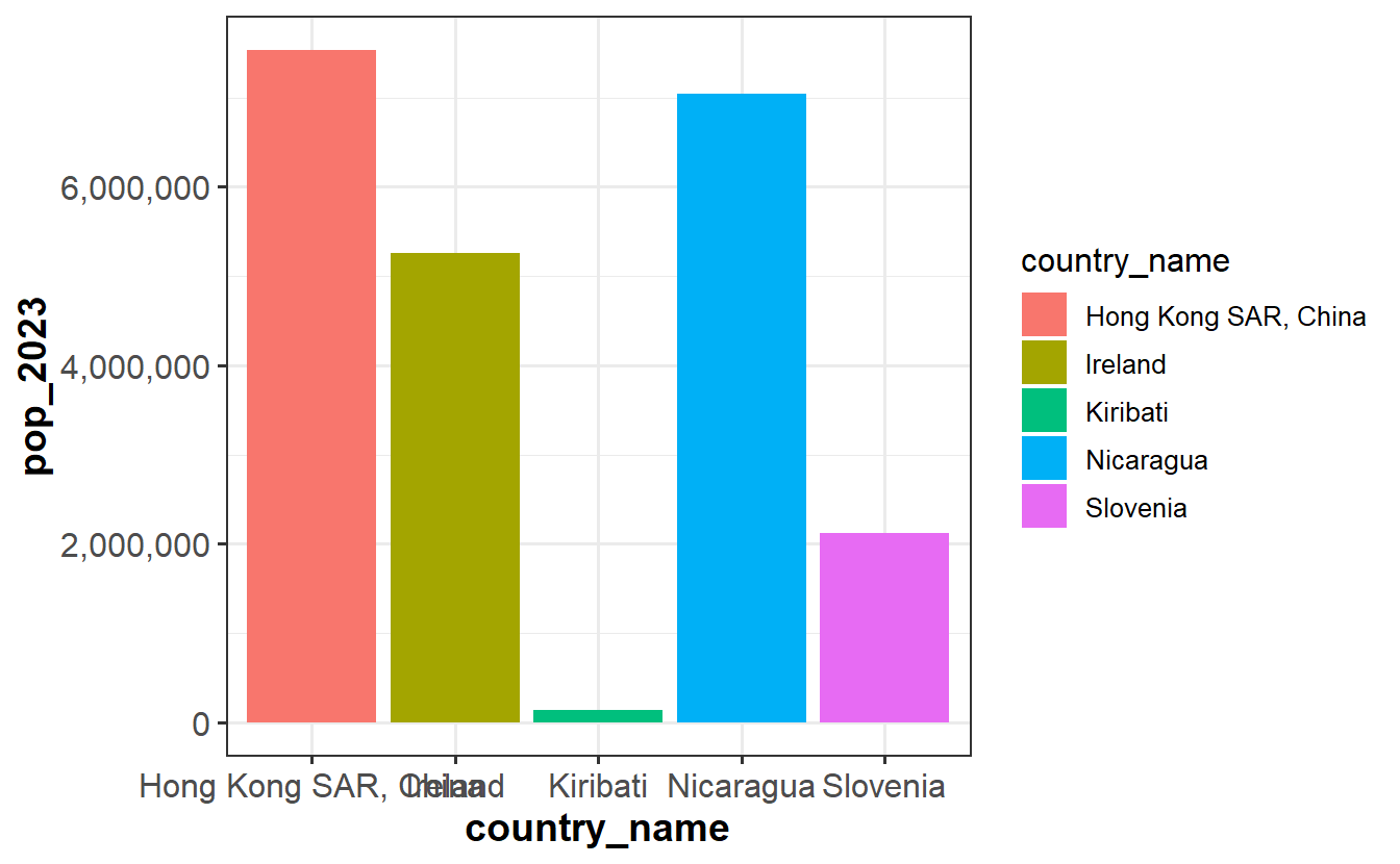
You are not impressed. List 5 specific things wrong with the plot above.
no title poor y-axis label poor x-axis label poor z-axis label could comment on color… unnecessary legend
Question 10b (3 points)
We want to calculate the mean of the pop_2023 column. Please write out the appropriate functions that should take the place of A1 and A2.
population |>
  A1(mean_pop = A2(pop_2023))
A1: summarise
A2: mean
Question 11
Aside: Classical music historians might disagree on the precise counts, but these values are widely accepted counts.
composers# A tibble: 6 × 3
composer genre count
<chr> <chr> <dbl>
1 Beethoven symphony 9
2 Beethoven opera 1
3 Beethoven concerto 9
4 Mozart symphony 41
5 Mozart opera 22
6 Mozart concerto 37Question 11 (3 points)
Just like addition and subtraction or multiplication and division, pivot_wider() and pivot_longer() are inverses. They undo each other.
Imagine we pivot the data frame composers given above, get it to the following format, and name it composers_pivoted:
composers_pivoted# A tibble: 2 × 4
composer symphony opera concerto
<chr> <dbl> <dbl> <dbl>
1 Beethoven 9 1 9
2 Mozart 41 22 37See next page for the rest of the question.
Which of the following will undo this transformation and give us back the original, composers, exactly?
composers_pivoted |>
  pivot_longer(
    cols = !composer,
    names_to = c("symphony", "opera", "concerto"),
    values_to = "count"
  )
composers_pivoted |>
pivot_longer(
cols = !composer,
names_to = "count",
values_to = c("symphony", "opera", "concerto")
)composers_pivoted |>
pivot_longer(
cols = !composer,
names_to = "count",
values_to = "genre"
)d.
composers_pivoted |>
  pivot_longer(
    cols = !composer,
    names_to = "genre",
    values_to = "count"
  )
End.