HW 2 - Data wrangling

Solutions

Homework

Important

This homework is due Monday February 10th.

Important

You may not earn more than a 100% on this assignment.

The first step in the process of turning information into knowledge process is to summarize and describe the raw information - the data. In this assignment we explore data on college majors and earnings, specifically the data begin the FiveThirtyEight story “The Economic Guide To Picking A College Major”.

These data originally come from the American Community Survey (ACS) 2010-2012 Public Use Microdata Series. While this is outside the scope of this assignment, if you are curious about how raw data from the ACS were cleaned and prepared, see the code FiveThirtyEight authors used.

We should also note that there are many considerations that go into picking a major. Earnings potential and employment prospects are two of them, and they are important, but they don’t tell the whole story. Keep this in mind as you analyze the data.

Workflow + formatting

Make sure to

Update author name on your document.
Follow the Tidyverse code style guidelines.
Make at least 3 commits.
Use informative labels for plot axes, titles, etc.
Turn in an organized, well formatted document.

Packages

We’ll use the tidyverse package for much of the data wrangling and visualization and the scales package for better formatting of labels on visualizations.

library(tidyverse)
library(scales)

Data

The data originally come from the fivethirtyeight package but we’ll use versions of the data that have been slightly modified to better suit this assignment. You can load the two datasets we’ll be using for this analysis with the following:

major_income_undergrad <- read_csv("data/major_income_undergrad.csv")
major_income_grad <- read_csv("data/major_income_grad.csv")

You can also take a quick peek at your data frames and view their dimensions with the glimpse function.

glimpse(major_income_undergrad)

Rows: 172
Columns: 12
$ major_code                            <dbl> 5601, 6004, 6211, 2201, 2001, 32…
$ major                                 <chr> "Construction Services", "Commer…
$ major_category                        <chr> "Industrial Arts & Consumer Serv…
$ undergrad_total                       <dbl> 86062, 461977, 179335, 37575, 53…
$ undergrad_employed                    <dbl> 73607, 347166, 145597, 29738, 43…
$ undergrad_employed_fulltime_yearround <dbl> 62435, 250596, 113579, 23249, 34…
$ undergrad_unemployed                  <dbl> 3928, 25484, 7409, 1661, 3389, 5…
$ undergrad_unemployment_rate           <dbl> 0.05066099, 0.06838588, 0.048422…
$ undergrad_p25th                       <dbl> 47000, 34000, 35000, 29000, 3600…
$ undergrad_median                      <dbl> 65000, 48000, 50000, 41600, 5200…
$ undergrad_p75th                       <dbl> 98000, 71000, 75000, 60000, 7800…
$ undergrad_sharewomen                  <dbl> 0.09071251, 0.69036529, 0.651659…

glimpse(major_income_grad)

Rows: 172
Columns: 11
$ major_code                       <dbl> 5601, 6004, 6211, 2201, 2001, 6206, 1…
$ major                            <chr> "Construction Services", "Commercial …
$ major_category                   <chr> "Industrial Arts & Consumer Services"…
$ grad_total                       <dbl> 9173, 53864, 24417, 5411, 9109, 19099…
$ grad_employed                    <dbl> 7098, 40492, 18368, 3590, 7512, 15157…
$ grad_employed_fulltime_yearround <dbl> 6511, 29553, 14784, 2701, 5622, 12304…
$ grad_unemployed                  <dbl> 681, 2482, 1465, 316, 466, 8324, 473,…
$ grad_unemployment_rate           <dbl> 0.08754339, 0.05775585, 0.07386679, 0…
$ grad_p25th                       <dbl> 110000, 89000, 100000, 85000, 83700, …
$ grad_median                      <dbl> 75000, 60000, 65000, 47000, 57000, 80…
$ grad_p75th                       <dbl> 53000, 40000, 45000, 24500, 40600, 50…

These two datasets have a trove of information. Three variables are common to both datasets:

major_code: Major code, FO1DP in ACS PUMS
major: Major description
major_category: Category of major from Carnevale et al

The remaining variables start with either grad_ or undergrad_ suffix, depending on which dataset they are in. The descriptions of these variables is as follows.

*_total: Total number of people with major
*_sample_size: Sample size (unweighted) of full-time, year-round ONLY (used for earnings)
*_employed: Number employed (ESR == 1 or 2)
*_employed_fulltime_yearround: Employed at least 50 weeks (WKW == 1) and at least 35 hours (WKHP >= 35)
*_unemployed: Number unemployed (ESR == 3)
*_unemployment_rate: Unemployed / (Unemployed + Employed)
*_p25th: 25th percentile of earnings
*_median: Median earnings of full-time, year-round workers
*_p75th: 75th percentile of earnings

Finally, undergrad_sharewomen is the proportion of women with the major, and we only have this information for undergraduates.

Let’s think about some questions we might want to answer with these data:

Which major has the lowest unemployment rate?
Which major has the highest percentage of women?
How do the distributions of median income compare across major categories?
How much are college graduates (those who finished undergrad) making?
How do incomes of those with a graduate degree compare to those with an undergraduate degree?

In the following exercises we aim to answer some of these questions.

Exercises

Exercise 1

Which majors have the lowest unemployment rate? Answer the question using a single data wrangling pipeline and focusing on undergraduates (major_income_undergrad). The output should be a tibble with the columns major, and undergrad_unemployment_rate, with the major with the lowest unemployment rate on top, and displaying the majors with the lowest 5 unemployment rates. Include a sentence listing the majors and the unemployment rates (as percentages).

major_income_undergrad |>
  arrange(undergrad_unemployment_rate) |>
  select(major, undergrad_unemployment_rate) |>
  slice_head(n= 5)

# A tibble: 5 × 2
  major                                      undergrad_unemployment_rate
  <chr>                                                            <dbl>
1 Geological And Geophysical Engineering                          0     
2 Educational Administration And Supervision                      0     
3 Pharmacology                                                    0.0179
4 Nuclear Engineering                                             0.0209
5 Treatment Therapy Professions                                   0.0217

Exercise 2

Which majors have the highest percentage of women? Answer the question using a single data wrangling pipeline and focusing on undergraduates (major_income_undergrad). The output should be a tibble with the columns major, and undergrad_sharewomen, with the major with the highest proportion of women on top, and displaying the majors with the highest 5 proportions of women. Include a sentence listing the majors and the percentage of women with the major.

major_income_undergrad |>
  arrange(desc(undergrad_sharewomen)) |>
  select(major, undergrad_sharewomen) |>
  slice_head(n = 5)

# A tibble: 5 × 2
  major                                         undergrad_sharewomen
  <chr>                                                        <dbl>
1 Early Childhood Education                                    0.969
2 Communication Disorders Sciences And Services                0.968
3 Medical Assisting Services                                   0.928
4 Elementary Education                                         0.924
5 Family And Consumer Sciences                                 0.911

Render, commit (with a descriptive and concise commit message), and push. Make sure that you commit and push all changed documents and your Git pane is completely empty before proceeding.

Exercise 3

How much are college graduates (those who finished undergrad) making? For this exercise, focus on undergraduates (major_income_undergrad).

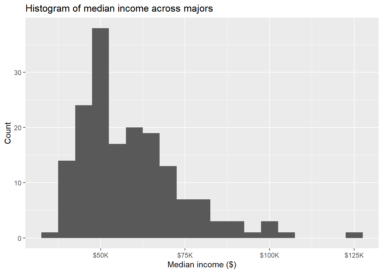
Plot the distribution of all median incomes using a histogram with an appropriate binwidth.

major_income_undergrad |>
  ggplot(
    aes(x = undergrad_median)
  ) +
  geom_histogram(binwidth = 5000) +
  scale_x_continuous(labels = label_dollar(scale = 1 / 1000, suffix = "K")) +
  labs(
    x = "Median income ($)",
    y = "Count", 
    title = "Histogram of median income across majors"
  )

Note: You can earn +2 extra credit points for using scale_x_continuous(), making the x axis have the appropriate $ label and units (K). Example: $50k.

This document may help under the section label currencies. Within label_dollar(), explore scale = and suffix =.

Calculate the mean and median for median income. Based on the shape of the histogram, determine which of these summary statistics is useful for describing the distribution. Justify your answer.

major_income_undergrad |>
  summarise(
    mean_ug = mean(undergrad_median),
    med_ug = median(undergrad_median)
  )

# A tibble: 1 × 2
  mean_ug med_ug
    <dbl>  <dbl>
1  58680.  55000

Describe the distribution of median incomes of college graduates across various majors based on your histogram from part (a) and incorporating the statistic you chose in part (b) to help your narrative. Hint: Mention shape, center, spread, any unusual observations.

*The distribution of median incomes of college graduates across various majors is right skewed, with a potential outliers at 125K. We observe the distribution to be right skewed because the mean is larger than the median, and we can see the right tail of the distribution be longer than the left.

Now is a good time to render, commit (with a descriptive and concise commit message), and push again. Make sure that you commit and push all changed documents and your Git pane is completely empty before proceeding.

Exercise 4

One of the sections of the FiveThirtyEight story is “All STEM fields aren’t the same”. Let’s see if this is true. Once again, focus on undergraduates (major_income_undergrad) for this exercise.

First, let’s create a new vector called stem_categories that lists the major categories that are considered STEM fields.
```
stem_categories <- c(
  "Biology & Life Science",
  "Computers & Mathematics",
  "Engineering",
  "Physical Sciences"
  )
```
Then, fill in the partial code to create a new variable in our data frame indicating whether a major is STEM or not. Note that you need to figure out the logical operator that goes into ___.
```
major_income_undergrad <- major_income_undergrad |>
  mutate(major_type = if_else(major_category ___ stem_categories, "STEM", "Not STEM"))
```

major_income_undergrad <- major_income_undergrad |>
  mutate(major_type = if_else(major_category %in% stem_categories, "STEM", "Not STEM"))

In a single pipeline, determine which STEM majors’ median earnings are less than $55,000. Your answer should be a tibble with the columns major, major_type, and undergrad_median, arranged in order of descending undergrad_median.

major_income_undergrad |>
  filter(
    major_type == "STEM",
    undergrad_median < 55000
  ) |>
  select(major, major_type, undergrad_median) |>
  arrange(desc(undergrad_median))

# A tibble: 7 × 3
  major                      major_type undergrad_median
  <chr>                      <chr>                 <dbl>
1 Biology                    STEM                  54000
2 Communication Technologies STEM                  52000
3 Botany                     STEM                  50000
4 Physiology                 STEM                  50000
5 Molecular Biology          STEM                  50000
6 Ecology                    STEM                  48700
7 Neuroscience               STEM                  40000

Once again, render, commit, and push. Make sure that you commit and push all changed documents and your Git pane is completely empty before proceeding.

Exercise 5

Finally, we want to compare median incomes of STEM majors with and without a graduate degree in their major.

To do so, we will first join data that contains information on median incomes of those with undergraduate and graduate degrees. Join the major_income_undergrad and the major_income_grad data sets by major_code. Join them in such a way where only rows that include the same major_code from each data set are included. Name the new data set major_income.

major_income <- major_income_undergrad |>
  inner_join(major_income_grad, by = c("major_code"))

Create a new variable called grad_multiplier – the ratio of median income of those with a graduate degree divided by median income of those with an undergraduate degree, for STEM majors. The result should be tibble with the variables major, grad_multiplier, grad_median, and undergrad_median. The results should be displayed in descending order of grad_multiplier and display the STEM majors with top 10 grad_multiplier.

major_income |>
  filter(major_type == "STEM") |>
  mutate(grad_multiplier = grad_median / undergrad_median) |>
  select(major.x, grad_multiplier, grad_median, undergrad_median) |>
  arrange(desc(grad_multiplier)) |>
  slice(1:10)

# A tibble: 10 × 4
   major.x                          grad_multiplier grad_median undergrad_median
   <chr>                                      <dbl>       <dbl>            <dbl>
 1 Zoology                                     2         110000            55000
 2 Physiology                                  1.8        90000            50000
 3 Biology                                     1.76       95000            54000
 4 Biochemical Sciences                        1.75       96000            55000
 5 Cognitive Science And Biopsycho…            1.73       95000            55000
 6 Molecular Biology                           1.7        85000            50000
 7 Chemistry                                   1.67      100000            60000
 8 Pharmacology                                1.59      105000            66000
 9 Geosciences                                 1.55       90000            58000
10 Oceanography                                1.5        90000            60000

Render, commit, and push one last time. Make sure that you commit and push all changed documents and your Git pane is completely empty before proceeding.

Wrap up

Submission

Go to http://www.gradescope.com
Click on the assignment, and you’ll be prompted to submit it.
Mark all the pages associated with exercise. All the pages of your homework should be associated with at least one question (i.e., should be “checked”). If you do not do this, you will be subject to lose points on the assignment.
Do not select any pages of your PDF submission to be associated with the “Workflow & formatting” question.

Grading

Exercise 1: 5 points
Exercise 2: 5 points
Exercise 3: 9 points
Exercise 4: 6 points
Exercise 5: 8 points
Workflow + formatting: 5 points
Total: 38 points