HW 5 - Modelling: Solutions

Homework

Packages

We’ll use the tidyverse package for much of the data wrangling and visualization, though you’re welcomed to also load other packages as needed.

library(tidyverse)
library(tidymodels)
library(openintro)

Data

For this homework, we are interested in the impact of smoking during pregnancy.

We will use the dataset births14, included in the openintro loaded at the beginning of the assignment. This is a random sample of 1,000 mothers from a data set released in 2014 by the state of North Carolina about the relation between habits and practices of expectant mothers and the birth of their children. Please, look at help(births14) for the variables contained in the dataset.

We are going to create a version of the births14 data set that drops NA values for the variable name habit. We are saving this as a new data set called births14_habitgiven. This will be the data set we use moving forward.

births14_habitgiven <- births14 |>
  drop_na(habit) #drop_na drops na values for just a single col

Exercise 1

model1 <- lm(weight ~ mage, data = births14_habitgiven)
summary(model1)


Call:
lm(formula = weight ~ mage, data = births14_habitgiven)

Residuals:
    Min      1Q  Median      3Q     Max 
-6.4598 -0.6449  0.1205  0.8250  3.1803 

Coefficients:
            Estimate Std. Error t value Pr(>|t|)    
(Intercept) 6.775362   0.207947  32.582   <2e-16 ***
mage        0.014979   0.007173   2.088    0.037 *  
---
Signif. codes:  0 '***' 0.001 '**' 0.01 '*' 0.05 '.' 0.1 ' ' 1

Residual standard error: 1.291 on 979 degrees of freedom
Multiple R-squared:  0.004435,  Adjusted R-squared:  0.003418 
F-statistic: 4.361 on 1 and 979 DF,  p-value: 0.03703

R fits this the “line of best fit” by fitting the line that minimizes the sums of squares residuals.
On average, when the mother’s age is 0, the estimated weight of the baby is estimated to be 6.78 pounds. This is clear extrapolation, as there is no data around a mother’s age of 0.

Note: Can also say “mean weight” instead of on average to reflect the response variable is a mean.

For a one year increase in mother’s age, we estimate on average, a 0.015 pound increase in the baby’s weight.

Note: Can also say “mean weight” instead of on average to reflect the response variable is a mean.

Exercise 2 - LEGO

lego_sample <- read_csv("data/lego_sample.csv")

r <- lego_sample |>
  summarize(r = cor(pieces, amazon_price))
r

# A tibble: 1 × 1
      r
  <dbl>
1 0.668

The correlation coefficient between the number of pieces of a Lego set and the price on Amazon is 0.6682458, indicating a rather moderate/strong positive linear relationship between the two variables.

s_price <- lego_sample |>
  summarize(s_price = sd(amazon_price)) 

s_piece <- lego_sample |>
  summarize(s_piece = sd(pieces)) 

s_price

# A tibble: 1 × 1
  s_price
    <dbl>
1    33.3

s_piece

# A tibble: 1 × 1
  s_piece
    <dbl>
1    214.

model2 <- linear_reg() |>
  fit(amazon_price ~ pieces, data = lego_sample)

model2_tidy <- tidy(model2)

The model estimates the following relation:

\[ \widehat{price} = 18.96 + 0.1*pieces \]

Note: They do not need to use LaTex to write this out. They should have something to indicate that this is an estimated response (hat).

We just want to save the slope coefficient from our model. However, instead of simply writing out the value, we know how to pull() it. Write the appropriate code to pull the slope coefficient from the model and save this as the r object slope.

$R^2$ = 0.447

slope <- model2_tidy |>
  filter(term == "pieces") |>
  pull(estimate)

To verify the relation, note that $\widehat{\beta_{piceces}}=0.104$ from the previous exercise and

r*s_price/s_piece

          r
1 0.1040297

slope

[1] 0.1040297

gives the same value, thus the relation is verified.

Exercise 3 - LEGO

lego_sample |>
  ggplot(aes(x=pieces, y=amazon_price, col=theme)) +
  geom_point() + 
  geom_smooth(method = "lm", se = F) +
  labs(x = "Number of Pieces", y = "Amazon Price", col = "Theme", 
       title = "Amazon Price and Number of Pieces of Lego Sets by Theme")

`geom_smooth()` using formula = 'y ~ x'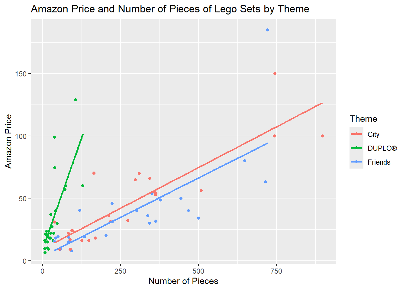

Note: They do not have to take the se bars off, but I anticipate most will, as this is what we have done in class.

From the plot it seems that across all sets, the Price increases as the number of pieces does. However, it seems that how much the price increases for the same increase in the number of pieces varies across the three themes. In particular, the steepest increase seems to happen for Lego Duplo, then for Lego City and lastly for Lego Friends.

model3 <- lm(amazon_price ~ pieces + theme, data = lego_sample)
summary(model3)


Call:
lm(formula = amazon_price ~ pieces + theme, data = lego_sample)

Residuals:
    Min      1Q  Median      3Q     Max 
-34.068 -12.736  -5.623   6.056  87.219 

Coefficients:
             Estimate Std. Error t value Pr(>|t|)    
(Intercept)   8.52364    6.14050   1.388  0.16945    
pieces        0.13380    0.01482   9.025 2.11e-13 ***
themeDUPLO®  21.10939    7.41084   2.848  0.00574 ** 
themeFriends -7.35361    6.50107  -1.131  0.26180    
---
Signif. codes:  0 '***' 0.001 '**' 0.01 '*' 0.05 '.' 0.1 ' ' 1

Residual standard error: 22.98 on 71 degrees of freedom
Multiple R-squared:  0.543, Adjusted R-squared:  0.5237 
F-statistic: 28.12 on 3 and 71 DF,  p-value: 4.281e-12

For a 1 piece increase in the number of pieces, we estimate on average a $0.134 increase in amazon price, after holding theme constant.

Note: Can also say “mean price” instead of on average to reflect the response variable is a mean.

$\hat{price} = 8.52 + .13*pieces - 7.35$

$\hat{price} = 1.17 + .13*pieces$

predict(model3, data.frame(pieces = 50, theme = "Friends"))

       1 
7.859872